Capacity Scaling of Wireless Networks with Inhomogeneous Node

1

Capacity Scaling of Wireless Networks with Inhomogeneous Node Density: Lower Bounds Giusi Alfano∗

Michele Garetto †

Emilio Leonardi ∗

Abstract— We consider static ad hoc wireless networks comprising significant inhomogeneities in the node spatial distribution over the area, and analyze the scaling laws of their transport capacity as the number of nodes increases. In particular, we consider nodes placed according to a shot-noise Cox process, which allows to model the clustering behavior usually recognized in large-scale systems. For this class of networks, we propose novel scheduling and routing schemes which approach previously computed upper bounds to the per-flow throughput as the number of nodes tends to infinity.

clusters) tends to infinity. The obtained results get close (up to a poly-log factor) to the upper bounds derived in a separate paper [7] in all scenarios in which the system throughput is limited by interference among concurrent transmissions.

I. I NTRODUCTION AND RELATED WORK In their seminal work, Gupta and Kumar [1] evaluated the capacity of a static ad-hoc wireless network consisting of n nodes randomly placed over a finite bi-dimensional domain and communicating among them (possibly in a multi-hop fashion) over point-to-point wireless links subject √ to mutual interference. They derived an upper bound1 of O(1/ n) to the per-node throughput, valid for arbitrary network topologies. In the case of nodes uniformly distributed over √ the network area, they proposed a scheme achieving Θ(1/ n log n) pernode throughput. Later on, Franceschetti at al.√[2] have applied percolation theory results to show that Θ(1/ n) transmission rate is achievable by the nodes also under uniform node placement. The goal of our work is to extend the capacity scaling analysis to networks characterized by large inhomogeneities in the node density over the area. Indeed, almost all large-scale structures created by human or natural processes over geographical distances (such as urban or sub-urban settlements) exhibit significant degrees of clustering, due to spontaneous aggregation of the nodes around a few attraction points. For example, many growing processes result into highly clustered networks due to preferential attachment phenomena. This fact motivated us to consider a general class of clustered point processes referred to as shot-noise Cox processes [3], which includes several special cases widely used in different fields, such as Neyman-Scott process [4], Mat´ern cluster process [5], Thomas process [6]. In this paper we introduce and analyze a class of scheduling and routing schemes specifically tailored to clustered random networks, deriving constructive lower bounds to the per-node throughput as the number of nodes (and the number of

To the best of our knowledge, only a few works have analyzed the capacity of clustered networks, especially departing from the assumption that nodes are uniformly placed over the network area. In [8], Toumpis considers a set of n nodes wishing to communicate to m = Θ(nd ) cluster heads, and points out that the network throughput can be limited by the formation of bottlenecks at the clusters heads. Both sources and cluster heads are uniformly distributed, so the overall node density does not exhibit inhomogeneities.

G. Alfano and E. Leonardi are with Dipartimento di Elettronica, Politecnico di Torino, Italy; M. Garetto is with Dipartimento di Informatica, Universit`a di Torino, Italy. 1 Given two functions f (n) ≥ 0 and g(n) ≥ 0: f (n) = o(g(n)) means limn→∞ f (n)/g(n) = 0; f (n) = O(g(n)) means lim supn→∞ f (n)/g(n) = c < ∞; f (n) = ω(g(n)) is equivalent to g(n) = o(f (n)); f (n) = Ω(g(n)) is equivalent to g(n) = O(f (n)); f (n) = Θ(g(n)) means f (n) = O(g(n)) and g(n) = O(f (n)); at last f (n) ∼ g(n) means limn→∞ f (n)/g(n) = 1

The main finding of this paper is that, in order to approach the existing upper bound to the per-node throughput, it is necessary to employ scheduling and routing schemes which are significantly more involved than the ones proposed for networks with homogeneous node density [2].

The deterministic approach proposed in [9] allows to derive capacity results also for some non-uniform node distributions. √ In particular, the authors√consider nodes distributed over n lines, or clustered into n neighborhoods. In both cases, a regular square tessellation of the network area can be built in such a way that no squarelet is empty w.h.p. (with high probability), while the maximum number of nodes in each squarelet increases at most as a poly-log function of n. Therefore, the network does not contain significant inhomogeneities, and the resulting capacity is similar to that derived by Gupta and Kumar. In [10] the authors consider a system which contains many circular clusters with uniform node density within them, whose centers are distributed according to a Poisson process over the network area (a Mat´ern cluster process). Moreover, clusters are surrounded by a sea of nodes with much lower node density. The only quantity that scales with n is the network size: below a critical network size, the per-node throughput is limited by the amount of data that a cluster can exchange with the sea of nodes, whereas above the critical size the per-node throughput is limited by the capacity of the sea of nodes. In contrast to [10], we consider a more general shot-noise Cox process, and we let the density of clusters (and the number of nodes per cluster) to scale with n as well. Moreover our scheduling and routing schemes are different. In [11] the authors present a spatial framework to upper bound the number of simultaneous transmissions in a network with general topology. However, their approach cannot be used to devise constructive schemes achieving the available per-node throughput for the class of networks considered here.

2

II. S YSTEM A SSUMPTIONS

AND

N OTATION

A. Network Topology We consider networks composed of a random number N of nodes (being E[N ] = n) distributed over a square region O of edge L. To avoid border effects, we consider wraparound conditions at the network edges (i.e., the network area is assumed to be the surface of a bi-dimensional Torus). The network physical extension L is allowed to scale with the average number of nodes, since this is expected to occur in many growing systems. Throughout this work we will always assume that L = Θ(nα ), with 0 ≤ α ≤ 1/2. The clustering behavior of large scale systems is taken into account assuming that nodes are placed according to a shotnoise Cox process (SNCP). An SNCP can be conveniently described by the following construction. We first specify a point process C of cluster centres, whose positions are denoted by C = {cj }M j=1 , where M is a random number with average E[M ] = m. In the literature the centre points cj are also called parent or mother points. Each centre point cj in turn generates a point process of nodes whose intensity at ξ is given by qj k(cj , ξ), where qj ∈ (0, ∞) and k(cj , ·) is a dispersion density function, also called kernel, or shot. In the literature the nodes generated by each centre are also referred to as offspring or daughter points. The overall node process N is then given by the superposition of the individual processes generated by the cluster centres. The local intensity at ξ of the resulting SNCP is Φ(ξ) =

X

qj k(cj , ξ)

j

Notice that Φ(ξ) is a random field, in the sense that, conditionally over all (qj , cj ), the node process N is an (inhomogeneous) Poisson point process with intensity function Φ. We denote by X = {Xi }N i=1 the collection of nodes positions in a given realization of the SNCP. In this work we restrict ourselves to kernels k(cj , ·) which are invariant under both translation and rotation, i.e., k(cj , ξ) = k(kξ − cj k) depends only on the euclidean distance kξ − cj k of point ξ from the cluster centre cj . Moreover we assume that k(kξ − cj k) is a non-increasing, bounded R and continous function, whose integral O k(cj , ξ) dξ over the entire network area is finite and equal to 1. In practice, the kernels considered in our work can be specified by first defining a non-increasing continuous function s(ρ) such that R∞ 0 ρ s(ρ) dρ < ∞ and then normalizing it over the network area O: s(kξ − cj k) k(cj , ξ) = R O s(kζ − cj k) dζ Notice that in our R asymptotic analysis we can neglect the normalizing factor O s(kζ − cj k) dζ = Θ(1). Indeed, k(cj , ξ) = Θ(s(kξ−cj k)). Notice that, in order to have finite integral over increasing networks areas, functions s(ρ) must be o(ρ−2 ), i.e., they must have a tail that decays with the distance faster than quadratically. Under the above assumptions on the kernel shape, quantity qj equals the average number of nodes generated by cluster centre cj . We assume that all cluster centres generate on

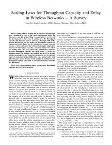
average the same number of nodes, hence qj = q = n/m. In our work, we let q scale with n as well (clusters are expected to grow in size as the number of nodes increases). This is achieved assuming that the average number of cluster centres scales as m = Θ(nν ), with ν ∈ (0, 1]. Consequently, the number of nodes per cluster scales as q = Θ(n1−ν ). At last we need to specify the point process C of cluster centres. We consider two different models: Cluster Grid Model. Clusters centres are deterministically placed over the vertices of a square grid. Cluster Random Model. Cluster centres are randomly placed according to a Homogeneous Poisson Process (HPP) of intensity φc = m/L2 . The Cluster Grid Model is simpler to analyze, because the overall node process turns out to be a standard inhomogeneous Poisson Point Process whose intensity over the area can easily be evaluated, since the clusters centres C are assigned. This model serves as an intermediate step towards the analysis of the more complex Cluster Random Model. √ For both models, we define dc = L/ m = Θ(nα−ν/2 ). This quantity represents, in the case of the Cluster Grid Model, the distance between two neighboring cluster centres on the grid; in the case of the Cluster Random Model, it is the edge of the square where the expected number of cluster centres falling in it equals to 1. We call cluster-dense regime the case α < ν/2, in which dc tends to zero an n increases. We call cluster-sparse regime the case α > ν/2, in which dc tends to infinity an n increases. Examples of topologies generated by our SNCP process can be found in [7]. Figure 1 shows three examples of the kind of topologies considered in this paper, in the case of n = 10, 000 and α = 0.25. In all three cases we have assumed s(ρ) = min(1, ρ−2.5 ). B. Communication Model We assume that time is divided into slots of equal duration, and that in each slot the scheduling policy enables a set of transmitter-receiver pairs to communicate over point-to-point wireless links which are modelled as Gaussian channels of unit bandwidth. We consider point-to-point coding and decoding, hence signals received from nodes other than the (unique) transmitter are regarded as noise. We assume that interference among simultaneous transmissions is described by the so called generalized physical model, according to which the rate achievable by node i transmitting to node j in a given time slot is limited to Rij = log2 (1 + SINRj ) where SINRj is the signal to interference and noise ratio at receiver j: P` P i ij SINRj = N0 + k∈∆,k6=i,j Pk `kj

Here, ∆ is the set of nodes which are enabled to transmit in the given slot, Pi is the power emitted by node i, `ij is the power attenuation between i and j, and N0 is the ambient noise power. In this paper we assume that all nodes employ the same power level while transmitting (i.e., Pi = P, ∀i). We remark that this assumption does not penalize the achievable throughput, as one can see by comparing our results with the

3

(a) Cluster Random model with ν = 0.6.

(b) Cluster Grid model with ν = 0.3.

(c) Cluster Random model with ν = 0.3.

Fig. 1. Examples of topologies comprising n = 10, 000 nodes distributed over the square 10 × 10 (α = 0.25). In all three cases s(ρ) ∼ ρ−2.5 . Case 1(a) belongs to the cluster-dense regime (α < ν/2). Cases 1(b) and 1(c) belong to the cluster-sparse regime (α > ν/2).

upper bounds in [7], which are derived for arbitrary power assignment. We further assume that the common power level P does not scale with n. The power attenuation is assumed to be a deterministic function of the distance dij between i and j, according to `ij = d−γ ij , with γ > 2. One drawback of this model is that the received power (and the corresponding rate) are amplified to unrealistic levels when dij tends to zero. Some authors have suggested to account for near-field propagation effect by bounding the attenuation function to 1: `ij = min{1, d−γ ij }. However, any fixed bound leads to pathological throughput degradation in network regions where the node density tends to infinity, as pointed out in [13]. To avoid such problems, we simply assume that the achievable rate on any link cannot grow arbitrarily large, but is bounded by a constant R0 due to the physical limitations of transmitters/receivers (maximum data speed of I/O devices, finite set of possible modulation schemes, etc). Therefore we consider the following variant of the generalized physical model: Rij = min{R0 , log2 (1 + SINRj )} while keeping `ij = d−γ ij , for any dij . The proposed interference model satisfies the following basic property. Lemma 1: Under the assumptions that, in a given time slot, i) every transmission take places between nodes whose relative distance is not greater than d; ii) the set ∆ of transmitters is chosen by the scheduling policy in such a way that the distance dij = ||Xi − Xj || between any two transmitters i,j in ∆ is greater than or equal to 3d; then the achievable rate by all concurrent transmissions during the considered slot is: R(d) = Ω(min[1, d−γ ]) Proof: The proof of this lemma, omitted for the sake of brevity, follows similar ideas as in the proof of Theorem 3 in [2].

C. Traffic Model Similarly to previous works [1], [2] we focus on permutation traffic patterns, i.e., traffic patterns according to which every node is source and destination of a single data flow at rate λ. Sources and destinations of data flows are randomly matched, establishing N end-to-end flows in the network. Note that a permutation traffic pattern is represented by a ˆ being Λ ˆ a permutation traffic matrix of the form Λ = λΛ matrix (i.e., a binary-valued doubly stochastic matrix). Let B(t) be the network backlog, that is, the number of data units already generated by sources which have not yet been ˆ is delivered to destinations at time t. We say that traffic λΛ sustainable if there exists a scheduling-routing policy such that lim supt→∞ B(t)/t = 0 almost surely. D. Asymptotic Analysis of network capacity We are essentially interested in establishing how the network capacity scales with n under the assumptions we have introduced above on network topology, communication model and traffic pattern. To summarize, the quantities that depend on n are: i) the network physical extension L = nα ; ii) the number of cluster centres m = nν , and consequently the average number q = n1−ν of nodes belonging to the same cluster. As the number of nodes increases, we generate a sequence of systems indexed by n. The per-node capacity is Θ(h(n)) if, given a sequence of random permutation traffic patterns with rate λ(n) = h(n), there exist two constants c, c0 such that c < c0 and both the following properties hold: ( limn→∞ Pr{cλ(n) is sustainable} = 1 limn→∞ Pr{c0 λ(n) is sustainable} < 1 Equivalently, we say in this case that the network capacity (or maximum network throughput) is Θ(nh(n)). To simplify the notation, in the following unless strictly necessary we will omit the dependence of the variables on n.

4

cluster-dense (LB=UB) Cluster Grid

√1 n

Cluster Random

√1 n

max

cluster-sparse (LB) «  √ „ L qs(dc ) 1 √ max R , n qs(dc ) ( q √ L

qs(dc n

log n)

R

1

q

qs(dc

√

ff

√

m R(dc ) n

!

log n)

,

)

√ m R(dc ) n

cluster-sparse (UB)  √ ff √ L qs(dc ) m max , log n n n

 √ ff √ L qs(dc ) log n m max , log n n n

TABLE I T HE PER - FLOW THROUGHPUT ACHIEVABLE IN DIFFERENT CASES . LB (UB) STANDS FOR L OWER B OUND (U PPER B OUND ).

III. S UMMARY OF R ESULTS Table III summarizes the maximum achievable per-flow throughput (in order sense) under the cluster dense (α < ν/2) and cluster sparse (α > ν/2) regimes, for both Cluster Grid and Cluster Random models. The table reports the lower bounds (LB) obtained in this paper, together with the corresponding upper bounds (UB) derived in [7]. We observe that the lower bound coincides with the upper bound in the cluster dense regime. In the cluster sparse regime, upper and lower bounds differ at most by a poly-log factor in the case of interference-limited systems (i.e., when R(d) = Θ(1), ∀d). Notice that upper bounds miss the terms R(·) since they assume arbitrary power levels (possibly scaling with n), which permit to compensate the effect of the attenuation function ` and thus achieve a fixed rate also between nodes whose relative distance diverges when n → ∞. IV. P RELIMINARIES Lemma 2: Consider a set of points X distributed over a bidimensional domain O of area L2 according to a HPP of rate Φ = n/L2 . Let A be a regular tessellation of O (or any sub-region of O), whose tiles Ak have a surface |Ak | non smaller than 16 logΦ n . Let U (Ak ) be the number of points of X falling within Ak . Then, uniformly over the tessellation, k| and 2Φ|Ak |, i.e., U (Ak ) is comprised w.h.p. between Φ|A 2 Φ|Ak | 2

< inf k U (Ak ) ≤ supk U (Ak ) < 2Φ|Ak |. The previous result can be immediately generalized to the case of Inhomogeneous Poisson Processes (IPP): Lemma 3: Consider a set of points X distributed over O according to a IPP having local intensity Φ(ξ), such that R Φ(ξ) dξ = n. Let A be any tessellation of O (or any O R sub-region of O), whose tiles Ak satisfy: Ak Φ(ξ) dξ ≥ 16 Rlog n. Then uniformly over the tessellations U (Ak ) = Θ( Ak Φ(ξ) dξ).

The following is a classical result on doubly stochastic matrices, known as the Birkhoff-von-Neumann (BvN) Theorem: Lemma 4: (BvN Theorem). Any doubly stochastic matrix can be decomposed into a convex combination of permutation matrices. From the BvN Theorem, it descends that every non-negative, integer-valued matrix A = [aij ] can be decomposed into the sum of at most H sub-permutation matrices (i.e., binary-valued P Pdoubly sub-stochastic matrices), being H = max( i aij , j aij ) the maximum column/row sum [12]. At last we report the main result of [2], together with a brief overview of their solution which allows us to make a trivial generalization of the same result. Lemma 5: Consider a set of nodes X placed according to a HPP with intensity Φ = 1 over domain O of area |O| =

n; then a scheduling/routing scheme exists such that the per√ node throughput is w.h.p. Θ(1/ n) under random permutation traffic. The scheduling/routing policy proposed in [2] exploits the formation of several horizontal and vertical paths across the network in the transition region of an underlying percolation model. Nodes along these paths form a highway system that can carry information using multiple hops of length Θ(1). The rest of the nodes √ access the highway system using single hops of length O( log n). The communication strategy is then divided into four consecutive phases: in a first phase, nodes drain their information to the highway, in a second phase information is carried horizontally across the network through the highway, in a third phase it is carried vertically, and in a last phase information is delivered from the highway to the destination nodes. The system bottleneck turns out to be due to the phases in which information is carried √ over the highway, hence the per-node throughput is Θ(1/ n). The previous scheduling/routing strategy can be extended to the more general case in which nodes are placed over a domain O of area |O| according to a HPP of rate Φ = n/|O|. Employing the same communication strategy as in [2], all√ distances covered by transmissions are scaled by a factor 1/ Φ. When Φ = Ω(1), the length of the hops along the highway system becomes o(1) (the distance √ between transmitters and receivers on the highway is Θ(1/ Φ)); the achievable rate on each hop along the highway remains Θ(1)√(see Lemma 1), hence the per-node throughput is still Θ(1/ n). When Φ = o(1), instead, the distances covered by transmissions along the highway become ω(1), √ and the corresponding rate over each hop degrades to R(1/ Φ) < 1 for effect of the noise power at the receiver (see again Lemma 1). As √ a result √ the per-node throughput reduces to Θ(1/ n R(1/ Φ)). V. A SYMPTOTIC ANALYSIS

OF THE LOCAL INTENSITY

Recall that, under both the Cluster Grid and the Cluster Random models, the local P intensity of nodes at point ξ can be written as Φ(ξ) = j qk(cj , ξ). For both models, we define the following two quantities: Φ = supO Φ(ξ) and Φ = inf O Φ(ξ). Under the Cluster Grid model, cluster centres are regularly placed in a deterministic fashion, hence Φ and Φ are two deterministic values depending only on system parameters. It is of immediate verification that, whenever dc = O(1), we have Φ = Θ(Φ) = Θ(n/L2 ). When dc = ω(1), Φ = o(Φ), being Φ = Θ(q s(dc )) and Φ = Θ(q). Under the Cluster Random model the computation of Φ and Φ is complicated by the fact that the local intensity of nodes Φ(ξ) is a random variable that depends on the cluster centres’

5

positions C. The following theorem characterizes the√extreme values of the local intensity as function of dc = L/ m. Theorem 1: Consider nodes distributed according to a √ Cluster Random model. Let η(m) = dc log m. If η(m) = o(1), then it is possible to find two positive constants g, G with g < G such that ∀ξ0 ∈ O n n g 2 < Φ(ξ0 ) < G 2 w.h.p. (1) L L which means that Φ = Θ(Φ). More in general, when η(m) = Ω(1) √ it results Φ = O(q log m) and Φ = Ω(q log m s(dc log m)). Proof: The proof of this theorem is reported in [7] The above results show that, for both Cluster Grid and Cluster Random models, Φ = Θ(Φ) in the cluster-dense regime (α < ν/2), whereas Φ = o(Φ) in the clustersparse regime (α > ν/2). In Section VI we analyze the case Φ = Θ(Φ) under both Cluster Grid and Cluster Random models. In Section VII we study the case Φ = o(Φ), separately considering the Cluster Grid and the Cluster Random models. VI. A NALYSIS OF THE CASE Φ = Θ(Φ) The scheduling/routing strategies we propose are based on the idea of extracting a subset of nodes forming an infrastructure through which data can be transported across the network. This subset of nodes is distributed on the area according to an HPP. The rest of nodes communicate with the infrastructure using single-hop transmissions. Lemma 6: If nodes X = {X}N 1 are placed either according to a Cluster Grid model or to a Cluster Random model and Φ = Θ(Φ) (cluster-dense regime), then a subset of nodes Z ⊆ X can be found with probability 1, such that: i) Z forms a HPP; ii) |Z| = Θ(n); iii) given a tessellation T of O with 2 n tiles Tj of area |Tj | = Ω( L log ), then, uniformly over the n tessellation, the number of points X falling in each tile is Θ( Ln2 |Tj |). Proof: Applying the thinning strategy described in Appendix I, we can extract from X a subset Z forming a HPP with intensity Φ; the average number of points belonging to Z is ΦL2 = Θ(n). Similarly, X can be completed to a HPP W of intensity Φ, by adding to X some extra points; the average number of points belonging to W is ΦL2 = Θ(n). From Lemma 2, setting |Tj | non smaller than 16 logΦ n we have that, uniformly over the tessellation, both the number of points of Z and the number of points of W in each tile are Θ( Ln2 |Tj |). The same is true also for points belonging to X, since Z ⊆ X ⊆ W. Theorem 2: Under the assumptions of Lemma 6, there exists a scheduling/routing scheme P achieving per-node √ throughput Θ(1/ n) as n → ∞. Proof: The proposed communication strategy is a generalization of the scheme introduced in [2]. Nodes in Z form the infrastructure carrying the traffic across the network area. Nodes in Y = X−Z send/receive data from the infrastructure by single-hop communications with a close-by node belonging to Z. More in details, we partition O into squarelets of area A = Θ(log n/Φ), with A > 16 log n/Φ, in which, according

to Lemma 2, there are at least bΦA/2c nodes belonging to Z. Recalling Lemma 6, the number of points W in each squarelet is upper-bounded by 2AΦ. Since, by construction, Y ⊆ X ⊆ W, any upper bound on the number of points W can be regarded as an upper bound on the number of points Y. We uniformly partition the nodes of Y falling in each squarelet into bΦA/2c groups, assigning each group to a different node of Z belonging to the same squarelet. By construction, each group contains at most d4Φ/Φe = Θ(1) nodes. Time is divided into regular frames, each one comprising three phases of equal duration. During the first phase, nodes in Y directly transmit to the node of Z assigned to the group they belong to. Lying both transmitter and receiver in the same squarelet, their relative distance d√ T is upper bounded by the diagonal of the squarelet: d ≤ 2A, being T p √ A = Θ(L log n/n).

To meet conditions of Lemma 1, transmissions occurring within the same squarelet, as well as transmissions √ occurring in squarelets containing points closer than 3 2A, are to be orthogonalized over time. To do this, the squarelets are partitioned into a finite number of subsets, each subset comprising regularly spaced, weakly-interferring squarelets. At any time only one subset of squarelets is activated, and at most one transmission is enabled in each activated squarelet (this approach to limit interference among concurrent transmissions is pretty standard in related work, see for example Theorem 3 in [2]). Applying Lemma 1, each enabled transmission can achieve a rate Ω(R(dT )). However, we have to consider the fact that in each squarelet there are O(log n) competing nodes belonging to Y. Since the fraction of time in which each of them can transmit scales as Ω(1/ log n), the achievable rate by each node of Y is Ω(R(dT )/ log n). During the second phase, data are transported by the infrastructure provided by nodes Z, either up to their final destination (if it belongs to Z), or to the node Z assigned to the group of the destination. For the analysis of the second phase, we just apply the result of [2], adopting their scheduling/routing technique (notice that the scheme in [2] is itself divided into 4 sub-phases, see Lemma 5). The only difference with respect to the assumptions of [2], relies on the fact in [2] a random permutation traffic pattern is assumed, in which each node is origin and destination of a single end-to-end flow established with a randomly selected destination. In our case, instead, during the second phase every node of Z pushes/pulls into/from the network infrastructure data belonging to (at most) d4Φ/Φe + 1 end-to-end flows. However, thanks to the BvN Theorem (see Lemma 4), we can decompose our traffic pattern into (at most) d4Φ/Φe + 1 permutation traffic patterns, and devote to each of them a finite fraction of the system bandwidth. Hence the result in [2] can be applied also to to our case: the infrastructure Z can transport the traffic injected by √ nodes in Y, as long as every end-to-end flow has rate O(1/ n). In the third phase, data are delivered from nodes in Z to their final destinations belonging to Y, through single-hop transmissions. The analysis of this phase is identical to that of the first phase, exchanging the role of transmitters and receivers.

6

√ Since R(dT )/ log n = ω(1/ n), the second phase acts as the√ system bottleneck, and the per-node throughput is Θ(1/ n). VII. A NALYSIS OF

THE CASE

Φ = o(Φ)

Recall that condition Φ = o(Φ) is verified only when dc = nα−ν/2 = ω(1) in the case of the Cluster Grid model, or dc = nα−ν/2 = Ω(1) in the case of the Cluster Random model. In this section we restrict our attention to the clustersparse regime (i.e., α > ν/2)2 . Note that condition α > ν/2 can occur only when m = o(n) (i.e., ν < 1). We distinguish two sub-cases: Φ = ω(1/d2c ) and Φ = O(1/d2c ), which are treated separately in Sections VII-A and VII-B, respectively. A. The cluster-sparse regime with Φ = ω(1/d2c ) Our approach is still based on the idea of extracting a subset Z of nodes distributed according to a HPP of intensity Φ, forming the infrastructure carrying data across the network. Since |Z| = o(n), we expect a throughput degradation with respect to the case Φ = Θ(Φ), in which |Z| = Θ(n). In principle, the rest of nodes could still access the above infrastructure through direct transmission, similarly to policy P. However, it turns out that this strategy is not always convenient, and can actually result in severe throughput degradation. This because in highly populated areas the density of nodes Z is negligible as compared to the density of nodes X. Hence the number of nodes Y = X − Z that would compete for transmission to the same node of Z can be very large (the number of competing nodes is Θ(Φ/Φ)), shifting the system bottleneck to the access phase (phase one), when: q  log n  L√Φ ΦR p  Φ =o R(1/ Φ) n Φ In this case, before accessing the infrastructure provided by Z, data originated by densely populated area needs to be spread out evenly on the network area. This is accomplished gradually, by covering highly dense areas of O with a hierarchy of intermediate, local transport infrastructures. Moving towards regions with higher and higher density, the area of such local infrastructures is reduced, while keeping their transport capacity approximately the same. Intermediate infrastructures allows to reduce the distance covered by transmissions in highly populated regions, while at the same time to efficiently balance the traffic towards the nodes of the main infrastructure. We start describing our solution for the Cluster Grid model, which is simpler to analyze, and later generalize our approach to the Cluster Random model. For the sake of simplicity and brevity, we assume that Φ = Ω(log n/d2c ), instead of Φ = ω(1/d2c ). However we remark that our results can be extended to the case Φ = o(log n/d2c ) by slightly modifying the adopted scheduling policy. 1) Cluster Grid Model: We build a sequence of nested domains Ok (for 0 ≤ k < Kmax = blog2 (Φ/Φ)c) according to the following definition: Ok = {ξ ∈ O : Φ(ξ) ≥ 2k Φ = λk }. Note that, by construction, Ok+1 ⊂ Ok , and O0 = O. 2 We

leave for future investigations the analysis of the limit case dc = Θ(1) for the Cluster Random model.

Symb. Ok Ick Ak Xk Zk Yk λk

Definition Layer-k infrstructure domain Layer-k isle around c Area of isles Ick Nodes within Ok Nodes within Ok forming the layer-k infrstructure Nodes within Ok − Ok+1 not belonging to Zk Spatial density of nodes Zk within Ok TABLE II S UMMARY OF NOTATION

Fig. 2. Example of construction of nested domains Ok for the Cluster Grid model for the topology of Figure 1(b).

Moreover, while O0 = O is by definition connected, domains Ok for k ≥ 1 are in general disconnected, being composed of m isolated domains Ikc , hereinafter called isles, of area Ak , surrounding each cluster centre:3 Ok = ∪c Ikc . We call pyramid the set of isles Ikc surrounding the same cluster centre c. Figure 2 shows an example of this construction. for the topology in Figure 1(b), characterized by Φ = 19, Φ = 4754, Kmax = 7. Notice that isles Ikc , k ≥ 1 have approximately a circular shape. We define by Xk the restriction of X on Ok ; i.e., Xk comprises all points of X lying in Ok . Applying the standard thinning procedure described in Appendix I to each domain Ok , a set of nodes Zk ⊆ Xk can be found such that: i) Zk is a HPP of intensity λk on Ok ; ii) any node belonging to Zk−1 and to Xk , also belongs to Zk , for k ≥ 1. Let Yk = Xk − (Xk+1 ∪ Zk ), i.e., Yk comprises those points of Xk lying in Ok − Ok+1 which do not belong to Zk . Table II summarizes the notation. Consider the following scheduling/routing scheme according to which time is partitioned into frames, each frame comprising Kmax + 1 descending phases 0, 1, . . . , Kmax followed by Kmax + 1 ascending phases 0, 1, . . . , Kmax . Each phase is in turn partitioned into two periods. Within descending phase Kmax − k (here index k runs from Kmax down to 0), during the first period all nodes in Yk are allowed to transmit their data to a close node in Zk within 3 We can formally define domain I c for any k ≥ 0 and c, as the set k of points of Ok whose closest cluster centre is c. According to this formal 2 definition A0 = L /m.

7

Ok ∈ Xi

1st period

(i > k)

∈ Yk

Ok−1

∈ (Zk − Zk−1 ) ∈ (Zk−1 ∩ Xk ) ∈ (Zk−1 − Xk )

2nd period Fig. 3.

∈ Yk−1

Illustration of descending phase Kmax − k.

the same pyramid, balancing the traffic among the candidate receivers. During the second period of the descending phase, nodes in Zk transmit to: i) randomly selected nodes lying within the same pyramid, and belonging to Zk ∩ Zk−1 , when k > 0; ii) randomly selected nodes belonging to Z0 ∩ Z1 , when k = 0. Nodes Zk transmit data gathered in the previous phase (if k < Kmax ), data gathered during the first period of the current phase, and their own data, again balancing the traffic among the feasible receivers. The data transport is achieved exploiting the scheme described in [2], on the infrastructure provided by Zk . Figure 3 illustrates the two periods of descending phase Kmax − k. In ascending phase k < Kmax , within the first period data directed to destinations in Xk − Xk+1 (i.e., lying in Ok but not in Ok+1 ) are transmitted exploiting the scheme in [2] on the infrastructure provided by Zk , either directly to their destination (whenever the destination belongs to Zk ) or to a close node in Zk , while at the same time, data directed to nodes lying within Ok+1 are routed to nodes of Zk ∩ Zk+1 lying within the same pyramid of the destination. During the second period of ascending phases k ≤ Kmax , data directed to nodes in Yk are delivered to their final destination through single-hop transmissions. Theorem 3: Under the assumption that λk Ak = Ω(αk λ0 A0 ), for some α > 1, the above described scheduling/routing scheme P1 for the√ Cluster Grid model sustains √a per-node throughput Θ(L Φ/n · R(d0 )), with d0 = 1/ Φ. Proof: Consider descending phase Kmax − k, √with 0 ≤ k ≤ Kmax . We fix the duration of this phase to 1/ αk , and suppose that the two periods within the same phase are of equal duration. Notice that, being α > 1, the total duration of all of the descending phases is bounded, although their number tends to infinity. We start looking at the first period of this phase, in which nodes in Yk are allowed to transmit to nodes in Zk lying in the same pyramid. We apply Lemma 3 to the network region Ok − Ok+1 (if k < Kmax , otherwise we take domain OKmax ), partitioning it into tiles T k having surface4 |T k | = 4 We shape the tiles in such a way that the maximum distance between two p points in the same tile T k is Θ( |T k |) for any k.

Θ(log n/λk ). Uniformly over the tiles, the number of points of Yk falling in each tile is O(log n), whereas the number of points of Zk in each tile is Ω(log n) (actually, there are Θ(log n) nodes of either sets in each tile). Hence we can apply the same approach already employed in the case Φ = Θ(Φ), assigning nodes Zk to nodes Yk residing within the same tile in such a way that the number of nodes Yk associated to the same node Zk is uniformly bounded by a constant. Also in this case, highly interfering transmissions are orthogonalized over time to meet conditions of Lemma 1: we adopt the same scheme used in the case Φ = Θ(Φ), partitioning tiles into a finite number of subsets, each comprising mutually weakly interfering tiles. Since the number of conflicting transmitters per tile is O(log n), √ the fraction of time devoted to each transmitter is Ω(1/(2 αk log n) and consequently √ the achievable T rate by every node in Yk is Ω(R(dk )/(2 αk log n), being p dTk = |T k |. In the second period, for k > 0, data are transported within isles Ick by nodes Zk , adopting again the scheme of [2]. We observe that, by construction, in each isle Ick the amount of data to be transferred is that generated by nodes lying within the same isle. The number of nodes belonging to the infrastructure covering Ick is zck = Θ(λk Ak ) (note that we are assuming that λk Ak = Ω(αk λ0 A0 ) being λ0 A0 = Ω(log n)). The total number of nodes nkc lying within Ick can be upper bounded as nkc = O(n/m) (note that n/m = ω(log n), as ν < 1). Since the capacity of√the infrastructure covering Ick is √ zk R(dk ), with dk = 1/ λk (see Lemma 5), and considering that such√infrastructure is used only for a fraction of time equal to 1/(2 αk ), the aggregate data rate that can √be sustained z R(d ) by the level-k infrastructure covering Ick is Ω( k√ k k ) = Ω(

√

2 α

λk Ak R(dk ) √ ). 2 αk

Thus, every node Zk is allowed to exchange √

with level-k infrastructure a data rate which is Ω( λk√AkkR(dk ) ). 2 α zk Considering that, by construction, every node of Zk is pushing/pulling into level-k infrastructure the aggregate data of O(nk /zk ) end-to-end flows, the achievable per-flow thoughput √ by level-k infrastructure is Ω( λk√AkkR(dk ) ) (to formally prove 2 α nk this result, we can resort to the trick of decomposing the traffic pattern into (sub)-permutation traffic patterns). When considering descending phase Kmax (k = 0), using similar arguments, it turns out that the achievable perflow √throughput by the ground√infrastructure (level-0) is: Θ(L Φ/n)R(d0 ), with d0 = 1/ Φ). Turning our attention to ascending phase k, we fix the √ duration of this phase to 1/ αk , and further assume that the two periods within the same phase are of equal duration. Then ascending phase k can be mapped to descending phase Kmax − k by reversing the time; i.e., observing the data transmission process backward. As a consequence the maximum throughput sustainable in ascending phase k equals the throughput sustainable in descending phase Kmax − k. We conclude that the maximum per-flow throughput sustainable by the whole system is given by the minimum among the per-flow throughput sustainable in every period of the frame. It turns out that the system bottleneck is again due to the capacity

8

Fig. 4. Example of construction of nested domains Ok for the Cluster Random model for the topology of Figure 1(c).

√ of the ground infrastructure, i.e., λ = Θ(L Φ/n)R(d0 ), with √ d0 = 1/ Φ). As final remark, we observe that the assumption λk Ak = Ω(αk λ0 A0 ) for some α > 1, is not restrictive. This property, indeed, can easily be verified to be equivalent to the condition that s(ρ) decreases asymptotically to zero faster than 1/ρ2+, for some  > 0. 2) Cluster Random model: Recall that (Theorem 1), in the cluster-sparse regime of the Cluster Random model, we have √ w.h.p. Φ = O(q log m) and Φ = Ω(q log m s(dc log m)). Moreover, using exactly the same arguments of Theorem 1, we can strengthen the upper bound on the local density at point ξ, provided that we know the distance between point ξ and the closest cluster centre, dmin (ξ) = minj ||ξ − cj ||. Then Φ(ξ) = O(qs(dmin (ξ)) log n). We employ a scheduling/routing scheme similar to the one devised for the Cluster Grid model. The main difference lies in the fact that, in the Cluster Random model, we have to deal with the irregular geometry induced by the random locations of the cluster centres. We define domains Ok , for k ≥ 1, as follows: Ok = {ξ ∈ k−1 O : dmin (ξ) ≤ dk = s−1 ( 2 q λ1 )}, with λ1 = q s(dc ), being  a small positive constant (again, conventionally, O0 = O). Note that the definition of Ok slightly differs from that introduced for the Cluster Grid model. Domains Ok are, in general, composed of many disjoint regions which are no longer associated through a one-to-one mapping to cluster centres cj . Indeed, several cluster centres can now fall within the same connected region (see Figure 4). Nevertheless, we will still denote by Ikj the k-th region to which cluster centre cj belongs to. Since domain Ok comprises all points whose distance from the closest cluster centre is smaller than threshold dk , regions Ikj are associated to the connected components of the standard Gilbert’s model of continuum percolation [15] with ball radius dk . The largest dk is d1 = dc . Choosing  sufficiently small, in such a way that the associated Gilbert’s model is below the percolation threshold (we need  < ∗ , where ∗ ≈ 0.6, [16]), we have the property that the maximum number of clusters centres belonging to the same region I1j is O(log n) w.h.p.

[17]. Since by construction Ok+1 ⊂ Ok , the same property holds for all k > 1. It follows that, in terms of physical extension, the area of region Ikj lies w.h.p. in the interval k−1 k−1 π(s−1 ( 2 q λ1 ))2 ≤ |Ikj | ≤ π(s−1 ( 2 q λ1 ))2 log n. In addition, by construction the density of nodes within Ok is lower bounded by λk = 2k−1 q s(dc ), for k ≥ 1. Hence, it is possible to define for every 0 ≤ k ≤ Kmax , (with Kmax = blog2 qs(0) λ1 c) a set of points Zk forming w.h.p. an HPP with intensity λk on Ok (in the case of k = 0, O0 = O and λ0 = Φ). Then we can apply the same scheme defined for the Clustered Grid model. The restriction of Zk to each Ikj corresponds to a level-k regional infrastructure covering Ikj , whose q √ aggregate capacity is λk |Ikj |R(1/ λk ); such capacity is exploited during descending phase Kmax −k (ascending phase k) to transport the information originated from (destined to) nodes lying on Ikj . Using the same arguments employed for the Cluster Grid model, we can prove that: 0 Theorem 4: Whenever s(ρ) decreases faster than 1/ρ2+ , 0 for some  > 0, the above described scheduling/routing scheme P2 for the √ Cluster Random model sustains √ a per-node throughput Θ(L Φ/n · R(d0 )), with d0 = 1/ Φ. B. The cluster-sparse regime with Φ = O(1/d2c ) When the minimal node density Φ drops below 1/d2c (in order sense) the approach of Section VII-A becomes suboptimal, because the ground level infrastructure provided by nodes Z0 (which determines the final network capacity) can be too sparse, especially when s(ρ) has a fast-decaying tail. In this case, considering first the Cluster Random model, a more dense set of nodes acting as ground-level infrastructure can be obtained by selecting one node per cluster; for example, according to an algorithm that selects for each cluster the closest node to the cluster centre. It is of immediate verification that the obtained set of nodes Z00 , forms a HPP, in light of the fact that: i) their number is distributed as a Poisson random variable with average m; ii) the positions of points Z00 are independent (since they belong to different clusters having independently located centres); iii) the marginal distribution of every point in Z00 is uniform over O since cluster centres are uniformly distributed over O. Note that, by construction, the density λ00 of Z00 is: λ00 = m/L2 = 1/d2c = ω(Φ). Then, defining domains Ok for k ≥ 1 according to: Ok = 2k λ0

{ξ ∈ O : dmin (ξ) ≤ s−1 ( q 0 )}, a simple variant of the scheme proposed in Section VII-A.2 permits to achieve higher throughput. We obtain the result: 0 Theorem 5: Whenever s(ρ) decreases faster than 1/ρ2+ , 0 for some  > 0, a scheduling/routing scheme P3 can be defined which √sustains a per-node throughput λ = Θ( dLc n R(dc )) = Θ( nm R(dc )). Turning our attention to the Cluster Grid model, by selecting one node per cluster according to the same algorithm proposed for the Cluster Random model, it is still possible to obtain a set Z00 of nodes providing a better ground-level infrastructure. In this case the set Z00 does not form a HPP. This fact, however, does not penalize the system performance, since

9

nodes in Z00 are almost regularly spaced (indeed, using standard concentration results it can be easily shown that, w.h.p., uniformly over the clusters, the distance between the selected node belonging to cluster j and the cluster centre cj is o(dc )). As a consequence, standard results [1], [9] can be invoked to √ conclude that Z00 provides an infrastructure of capacity Θ( m). Hence we obtain the same per-node throughput as in Theorem 5. VIII. C ONCLUSIONS In this paper, we have derived constructive lower bounds to the asymptotic capacity of static ad-hoc networks in which nodes are placed according to a Shot Noise Cox Process (SNCP). Such processes provide a fairly general model to capture the clustering behavior usually found in realistic largescale systems. The presented lower bounds differ at most by a poly-log factor from existing upper bounds, under the assumption that the system throughput is limited by interference among concurrent transmissions. Our study has revealed the emergence of two √ regimes: the cluster dense regime, where an optimal Θ(1/ n) per-node throughput is achieved, and the cluster sparse regime, where the per-node throughput degrades due to large inhomogeneities in the node spatial distribution. In the latter regime we have shown that the system throughput is intrinsecally related to the minimum node density within the network area. R EFERENCES [1] P. Gupta, P.R. Kumar, “The capacity of wireless networks”, IEEE Trans. on Inf. Theory, vol. 46(2), pp. 388–404, Mar. 2000. [2] M. Franceschetti, O. Dousse, D.N.C. Tse and P. Thiran, “Closing the gap in the capacity of random wireless networks via percolation theory,” IEEE Trans. on Inf. Theory, Vol. 53, No. 3, pp. 1009–1018, 2007. [3] Møller J., “Shot noise Cox processes,”, Adv. Appl. Prob. 35, 614–640, 2003. [4] J. Neyman and E. L. Scott, “Statistical approach to problems of cosmology,” J. R. Statist. Soc. B, Vol. 20, No. 1, pp. 1-43, 1958. [5] B. Mat´ern, “Spatial variation”, Lecture Notes in Statistics, vol. 36, second ed. Springer, Berlin, 1986. [6] M. Thomas, “A generalization of Poissons binomial limit for use in ecology”, Biometrika, Vol. 36, No. 1/2, pp. 18–25,1949. [7] G. Alfano, M. Garetto, E. Leonardi, “Capacity Scaling of Wireless Networks with Inhomogeneous Node Density: Upper Bounds”, http: //www.di.unito.it/˜garetto/papers/upper.pdf [8] S. Toumpis, “Capacity bounds for three classes of wireless networks: asymmetric, cluster, and hybrid”, ACM MobiHoc, pp. 133–144, Tokyo, Japan, May 2004 [9] S. R. Kulkarni, P. Viswanath, “A Deterministic Approach to Throughput Scaling in Wireless Networks”, IEEE Trans. on Information Theory, vol. 50, no. 6 , pp. 1041–1049, June 2004 [10] E. Perevalov, R. S. Blum, D. Safi, “Capacity of Clustered Ad Hoc Networks: How Large Is Large?,” IEEE Trans. on Communications, Vol. 54, No. 9, pp. 1672–1681, Sept. 2006. [11] A. Keshavarz-Haddad and R. H. Riedi, “Bounds for the capacity of wireless multihop networks imposed by topology and demand,” in Proc. ACM MobiHoc ’07, pp. 256–265, Montreal, Quebec, Canada, Sept. 2007. [12] T Weller, B, Hajek. “Scheduling Nonuniform Traffic in a PacketSwitching System with Small Propagation Delay”, IEEE/ACM Trans. on Networking, Vol.5(6), pp. 813–823, 1997. [13] O. Dousse and P. Thiran, “Connectivity vs capacity in dense ad-hoc networks, in Proc. INFOCOM, Hong Kong, 2004. [14] R. Motwani, P. Raghavan, Randomized algorithms, Cambridge University Press, 1995. [15] E. N. Gilbert, “Random plane networks,” J. SIAM, 9:533-543 (1961). [16] J. Quintanilla, S. Torquato, and R. M. Ziff, “Efficient measurement of the percolation threshold for fully penetrable discs”, J. Phys. A: Math. General, 33:L399-L407 (2000). [17] R. Meester and R. Roy, Continuum Percolation, Cambridge University Press. 1996.

A PPENDIX I T HINNING OF INHOMOGENEOUS POINT PROCESS First let us consider a set X = {X}N 1 of points distributed over a compact domain O according to an inhomogeneous Poisson process of intensity Φ(ξ). Let Φ be inf ξ∈O Φ(ξ). We need to show that for any Φ ≤ Φ a thinning procedure can be defined to extract a subset of points Z ⊆ X forming a homogeneous Poisson process of rate Φ. The thinning procedure works as follows: for each realization of X = {X}N 1 , consider each node, and mark it Φ with probability g(ξ) = Φ(ξ) , where ξ is the position of the node. The set of marked points form a Homogeneous Poisson Process with the desired intensity. Indeed consider a domain A ∈ O. Let U (A) be the random variable denoting the number of points of X falling within A ˆ (A) be the random variable denoting the number of and let U points of Z falling within A. Since, given the event {U (A) = i}, the i points of X falling in A are independently distributed over A according to the distribution R Φ(x) , it turns out that: Φ(x) dx A

ˆ Pr{U(A) = k | N (A) = i} = R   R g(ξ)Φ(ξ) dξ k  g(ξ)Φ(ξ) dξ i−k i AR = × 1 − AR = k Φ(ξ) dξ Φ(ξ) dξ A A   i  |A|φ k  |A|φ i−k R × 1− R (2) = k A Φ(ξ) dξ A Φ(ξ) dξ

Hence, unconditioning over i: ∞   X i |A|φ k ˆ R Pr{U(A) = k} = × k A Φ(ξ) dξ i=k i  R R   Φ(ξ) dξ i−k − A Φ(ξ) dξ |A|φ A × 1− R e = i! Φ(ξ) dξ A ∞ e−(|A|Φ ) −(R Φ(ξ) dξ−|A|φ) X 1 A = e × k! (i − k)! i=k Z i−k e−|A|φ × Φ(ξ) dξ − |A|φ = k! A

(3)

The above thinning procedure can be generalized so as to extract a subset of points Z ⊆ X forming a HPP, in the case in which the intensity of the original inhomogeneous point process is function of some random P parameter. More specifically, let Φ(ξ) = j k(cj , ξ) be a SNCP, being C = {cj }M 1 the cluster centres distributed according to a HPP of rate φc . Let again Φ = inf O Φ(ξ). Then a subset Z of nodes forming a HPP of rate Φ can be obtained from X, for any Φ ≤ Φ, by marking, conditionally over C, a point in ξ with a Φ (conditional) probability g(ξ | C) = P k(c . The fact that j ,ξ) j

the set of points Z so obtained is a HPP, can be proved in the same way as before, conditioning over C. Similar arguments can be used to show that a set of points X = {X}N 1 forming either a IPP or a SNCP with intensity Φ(ξ), such that Φ = supξ∈O Φ(ξ), can always be completed, by adding some extra points, to a set W ⊇ X, being W a HPP with intensity Φ ≥ Φ.