General Capacity Scaling of Wireless Networks - Computer Science

General Capacity Scaling of Wireless Networks Cheng Wang∗† , Xiang-Yang Li‡§ , Changjun Jiang∗† , Shaojie Tang‡ Department of Computer Science, Tongji University, Shanghai, China Key Laboratory of Embedded System and Service Computing, Ministry of Education, Shanghai, China ‡ Department of Computer Science, Illinois Institute of Technology, Chicago, IL, 60616 § TNLIST, School of Software, Tsinghua University ∗

†

Abstract—We study the general scaling laws of the capacity for random wireless networks under the generalized physical model. The generality of this work is embodied in three dimensions denoted by (λ ∈ [1, n], nd ∈ [1, n], ns ∈ (1, n]). It means that: (1) We study the random network of a general node density λ ∈ [1, n], rather than only study either random dense network (RDN, λ = n) or random extended network (REN, λ = 1) as in most existing works. (2) We focus on the multicast capacity to unify unicast and broadcast capacities by setting the number of destinations of each session nd ∈ [1, n]. (3) We allow the number of sessions changing in the range ns ∈ (1, n], rather than assuming that ns = Θ(n) as in most existing works. We derive the general lower and upper bounds on the capacity for the arbitrary case of (λ, nd , ns ). Particularly, when the general results are applied to the special cases (λ = 1, nd ∈ [1, n], ns = n) and (λ = n, nd ∈ [1, n], ns = n), we show that our results close the previous gaps between upper and lower bounds on the multicast capacity under the generalized physical model.

I. I NTRODUCTION We focus on the issue of capacity scaling laws for wireless networks that is initiated by Gupta and Kumar [1]. Most of the existing results differ from each other because of the diversity of analytical models and assumptions to be used. In terms of scaling patterns, there are two typical models adopted by many existing works: random extended network (REN), where the node density is fixed to a constant [2]–[5], and random dense network (RDN), where the node density increases linearly with the number of nodes [1], [6]–[9]. In the research of networking-theoretic capacity scaling laws [10], the unicast and broadcast sessions can usually be regarded as two special cases of multicast sessions according to the number of destinations of each session, denoted by nd : [1, n]1 . Then, any proposed multicast capacity could be specialized to the unicast and broadcast capacities by letting nd = 1 and nd = n. The literature [3], [5], [7], [9], [11], [12] all follow this criterion. In [7], Shakkottai et al. derived the multicast capacity of RDN for a specifical case that ns = n² and ns · nd = Θ(n), where ² ∈ (0, 1] and ns denotes the number of sessions (source nodes). They showed that such per-session multicast capacity under the protocol model is at most of order O( √n 1log n ). To achieve s the upper bound, they propose a simple and novel routing architecture, called the multicast comb, to transfer multicast data in the network. A more general result, in terms of ns 1 We use the term f (n) : [φ (n), φ (n)] to represent f (n) = Ω(φ (n)) 1 2 1 and f (n) = O(φ2 (n)); and use f (n) : (φ1 (n), φ2 (n)) to represent f (n) = ω(φ1 (n)) and f (n) = o(φ2 (n)).

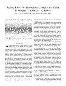
and nd , was proposed by Lipet al. in [11]. They showed that when ns = Ω(log nd · n log n/nd ), the per-session multicast capacity for RDN under the protocol model is of q n n order Θ( n1s nd log n ) if nd = O( log n ), and is of order Θ(1/ns ) if nd = Ω(n/log n). Later, Keshavarz-Haddad et al. [9] computed the multicast capacity for RDN under the generalized physical model [13]. They designed the multicast scheme by which the throughput can be achieved of the order as in Equation (2), and derived the upper bounds as in Equation (3). A gap remains open between the upper and lower bounds in the regime nd : [n/(log n)3 , n/ log n] (Please see the illustration in Fig.1(a)). For multicast capacity of REN under the generalized√physical model, Li et al. [3] derived a lower bounds as Ω( ns √nnd ) for the case that ns = Ω(n1/2+² ) and nd = O(n/(log n)2α+6 ). Recently, Wang et al. [5] devised the specific multicast schemes and derived the multicast throughput for all cases ns : (1, n] and nd : [1, n]. Under the assumption that ns = Θ(n), their lower bounds are specialized into that in Equation (4). They also derived an upper bounds for the case that ns = Θ(n), as in Equation (5). An obvious gap exists between the upper and lower bounds in the regime nd : [n/(log n)α+1 , n/ log n] (Please see the illustration in Fig.1(b)). Closing these gaps is one of the motivations of this paper. Both REN and RDN are two extreme cases for a random network of size (the number of nodes, n) in terms of the node density λ. The characterization of two particular models does not suffice to develop a comprehensive understanding of wireless networks, although they are representative models to some extent, [10]. Hence, in this paper, we consider comprehensively the network with a general node density λ : [1, n], rather than only the cases λ = 1 (REN) and λ = n (RDN), which can offer complete and deep insights about the scaling laws for wireless networks. Unearthing the nature of general scaling is the other motivation of this work. We aim to examine the capacity scaling laws of general wireless networks, where the generality is embodied in three dimensions (represented by (λ, nd , ns )): (1) general node density λ : [1, n]; (2) general number of receivers nd : [1, n]; (3) general number of sessions ns : (1, n]. Main Contributions: We now summarize major contributions of this paper as follows: •

For computing lower bounds of multicast capacity under the generalized physical model, we build two levels of

2

routing backbones: highways and arterial roads. Furthermore, arterial roads (ARs) have two subclasses, i.e., ordinary arterial roads (O-ARs) and parallel arterial roads (P-ARs). Notice that the highways are the same as that in [2], [3], [5], [9], but the ARs are different from the second-class highways (SHs) in [5]. Recall that in the SH system of [5], there are two types of SHs: odd SHs and even SHs. The bottlenecks of the whole routing could happen in the switching phase between the odd and even SHs. There is no such bottleneck in the current AR system, which can improve the multicast throughput for some regimes of ns and nd . Based on the highways, O-ARs and P-ARs, we design four routing schemes. By exploiting the theory of maximum occupancy, we derive the optimal multicast throughput and scheme according to different ranges of λ, nd , and ns . • For deriving upper bounds on multicast capacity, we introduce the Poisson Boolean model of continuum percolation [14] (not Poisson bond percolation model [2]), which, to the best of our knowledge, is not used in previous studies on upper bounds of network capacity. Based on the argument of giant cluster (component) in the Poisson boolean percolation model, we can divide the communications under any multicast routing scheme into two parts, i.e., communications inside and outside the giant cluster. Obviously, the network throughput must be determined by the bottleneck of two parts. We give a general formula to compute upper bounds on the capacity. • For the case that ns = Θ(n) and λ = n (or λ = 1), i.e., RDN and REN, due to the limitations of adopted analyzing methods, the previous works [5], [9] have not derived the tight bounds on multicast capacity under the generalized physical model. By adopting our general results to these special cases, we close these gaps. The rest of the paper is organized as follows. The system model is formulated in Section II. We present and discuss the main results in Section III. We derive the lower and upper bounds on the capacity in Section IV and Section V, respectively. Finally, we draw some conclusions in Section VII. II. S YSTEM M ODEL A. Random Network Model We construct a random network, denoted by N (λ, n), with node density λ by placing n nodes randomly and √ uniformly into a square deployment region R(λ, n) = [0, A]2 , where A = n/λ. When λ is set to be 1 (or n), our model corresponds to the random extended network (REN) (or random dense network (RDN)). Denote the set of all n nodes by V := V(n), and choose uniformly ns nodes to form a subset, denoted by S := S(ns ), in which every node acts as the source of a multicast session. For every source k ∈ S, choose uniformly nd nodes at random from all other nodes to form a subset, denoted by Dk , that acts as the set of destinations of the source k. We denote such a session with the source k by Mk , and define Uk := {k} ∪ Dk as the spanning set of Mk .

We follow the formal definitions of capacity in [1], [11]. Due to limited space, we omit the detailed introduction for those definitions. Please refer to the detailed definition of throughput capacity in [1] (Page 3) and Definition 2 of [11]. B. Communication Model Generally, there are three types of communication (interference) models: the protocol model [1], physical model [1] and generalized physical model [13]. We adopt the generalized physical model because it is more realistic than the other two ones [2], [3], [8], [13]. Let Kt denote a scheduling set of links in which all links can be scheduled simultaneously in time slot t. Specifically, Definition 1: Under the generalized physical model, when a scheduling set Kt is scheduled, the rate of a link < u, v >∈ Kt is achieved of Ru,v;t = B × 1 · {< u, v >∈ Kt } × log(1 + SINRu,v;t ), (1) P ·`(|xu −xv |) where SINRu,v;t = N0 +P ; xu de∈Kt / P ·`(xi −xv |) notes the position of node u, |xu − xv | represents the Euclidean distance between node u and node v; `(·) denotes the power attenuation function that is assumed to depends only on the distance between the transmitter and receiver [1]– [3], [15]; `(| · |) := | · |−α for dense scaling networks, and `(| · |) := min{1, | · |−α } for extending scaling networks [2].

III. M AIN R ESULTS We derive the general capacity scaling laws of random ad hoc networks. A. General Lower Bounds Theorem 1: The multicast throughput for random network N (λ, n) can be achieved of order Λ(λ, n) = max{Λo (λ, n), Λp (λ, n), Λo&h (λ, n), Λp&h (λ, n)}, where Λo (λ, n), Λp (λ, n), Λo&h (λ, n), Λp&h (λ, n) are defined in Table.I. B. General Upper Bounds Theorem 2: The multicast capacity for random network N (λ, n) is at most of      min{1, l−α } min{1, ( λ ) α2 }  log n c √ √ , Λ(λ, n) = max min ,  L(ns , √ n ) L(ns , n· √λ·lc )  lc :Lc  l n λ n · log n c

d

d

√ p where Lc = [1/ λ, log n/λ]. C. Tight Capacity Bounds When ns = Θ(n) In this section, we specialize the general results from Theorem 1 and Theorem 2 to the cases that λ = n and λ = 1, corresponding to the RDN and REN. Following a common assumption in most existing work, i.e., ns = Θ(n), we show that for both RDN and REN our results give the first tight bounds on multicast capacity over the whole regime nd : [1, n].

3

1) Random Dense Networks: In Theorem 2, Λ(n, n), i.e., the upper bound on the capacity, achieves the maximum by choosing lc = Θ( √1n ) when nd = O(n/(log n)2 ); and √ √ achieves the maximum by choosing lc = Θ( log n/ n) 2 when nd = Ω(n/(log n) ). Specifically, the multicast capacity is at most of order  when nd : [1, (lognn)3 ] Θ( √n1d n )    1  Θ( when nd : [ (lognn)3 , (lognn)2 ] 3 ) nd (log n) 2 (2)  Θ( √nn 1 log n ) when nd : [ (lognn)2 , logn n ]   d  Θ( n1 ) when nd : [ logn n , n]

TABLE I D EFINED F UNCTIONS AND PARAMETERS . Functions Λo (λ, n) Λp (λ, n) Λo&h (λ, n) Λp&h (λ, n)

L(m, n)

It is easy to see that there is a gap between the upper and lower bounds in the regimes nd : ( (lognn)3 , logn n ). Please see the illustration in Fig.1(a). In this work, we close this gap. Moreover, by Theorem 1, this optimal throughput in Equation (2) can also be achieved by using cooperatively our schemes Mo and Mo&h that are defined in Table.II. 2) Random Extended Networks: In Theorem 2, Λ(1, n) in Theorem 2 achieves the maximum by letting lc = Θ(1) when nd = O(n/(log n)2 ); and achieves the maximum by letting √ lc = Θ( log n) when nd = Ω(n/(log n)2 ). Specifically, the multicast capacity is at most of order  n Θ( √n1d n ) when nd : [1, (log n)  α+1 ]    n n 1  ) when n : [ Θ(  α+1 d (log n)α+1 , (log n)2 ]

RH (λ, n)

nd (log n)

2

nd (log n)

nd : [ (lognn)2 , logn n ]

1 ) po 1 RP−AR (λ, n)/L(ns , p ) p (

RO−AR (λ, n)/L(ns ,

min (

This result is exciting, because the multicast throughput as in Equation (2) had been proven to be achievable by Keshavarz-Haddad et al. in [9]. While, they derived an upper bound as  1 when nd : [1, (lognn)2 ]   O( √nd n ) 1 O( nd ·log n ) when nd : [ (lognn)2 , logn n ] (3)  n  O( 1 ) when n : [ , n] d n log n

1 when Θ( √ α−1 )   nnd ·(log n) 2    1  Θ( when α ) 2

Definitions

RO−AR (λ, n)

RP−AR (λ, n)

po

pp

poh,O−AR

poh,H , pph,H pph,P−AR

)

RO−AR (λ,n) RH (λ,n) , 1 L(ns , p ) L(ns , p 1 ) oh,O−AR

oh,H

)

RP−AR (λ,n) RH (λ,n) , 1 L(ns , p ) L(ns , p 1 )

min ph,H  ³ ´ph,P−AR log n n  when m : [1, polylog(n) ) Θ  n   ¶ µlog m  log n n Θ when m : [ polylog(n) , n log n) n  log n log  m  ¡ ¢   Θ m when m = Ω(n log n) n  α   Θ( λ 2 α ) when λ : [1, log n] (log n) 2

  Θ(1)  α   Θ( λ 2  

α

(log n) 2 Θ( log1 n )

)

when

λ : [log n, n]

when

λ : [1, (log n)1− α ]

when

λ : [(log n)1− α , n]

2

2

Θ(1) for all λ : [1, n]  q  Θ( nd log n ) when n = O( n ) d n log n n  Θ(1) when nd = Ω( log ) n  √ n  Θ( √ d ) when n : [1, n ] d log n n log n n  Θ( nd ) when n : [ , n] d n log n  3/2 n ·(log n) n d  Θ( ) when nd : [1, n

(log n)3/2

]

n  Θ(1) , n] when nd : [ (log n)3/2  q nd n  Θ( n ) when nd : [1, (log n)2 ]    nd log n n Θ( n ) when nd : [ (lognn)2 , log ] n     Θ(1) n when nd : [ (log , n] n)  √  Θ( nd · log n ) when nd : [1, √ n ] n log n

 Θ(1)

n when nd : [ √log , n] n

nd : [ logn n , n]

(4) Also, such multicast throughput had been achieved by the schemes in [5]. The upper bounds were proposed as: ( O( √n1d n ) when nd : [1, (lognn)α ] (5) 1 when nd : [ (lognn)α , n] O( α ) 2 nd (log n)

Successfully, we close the gap between the upper and lower n n bounds in the regime nd : [ (log n) α+1 , log n ] that is illustrated in Fig.1(b). In addition, by Theorem 1, this optimal throughput in Equation (4) can be equally achieved by using cooperatively our schemes Mp and Mp&h that are defined in Table.II. IV. L OWER B OUNDS ON M ULTICAST C APACITY We derive the lower bounds on multicast capacity by proposing four multicast schemes. Our multicast schemes are cell-based, then we first recall a notion called scheme lattice from [16] for succinctness of the description. Definition 2 (Scheme Lattice): Divide the deployment rep gion R(λ, n) = [0, n/λ]2 into a lattice consisting of square

cells of side lengthpb, we call the lattice scheme lattice and denote it by L( n/λ, b, θ), where θ ∈ [0, π/4] is the minimum angle between the sides of the deployment region and produced cells. In our multicast schemes, the backbones of routing contain two levels: the highway system and arterial road system. A. Highway System The highway system is built in [2] based on bond percolation theory [17]. For completeness, we introduce concisely the procedure of construction in [2], and extend the related results in [2] into the scenario with general node density by a simple geometric scaling. Construction of highway system:pThe highways are p built based on the scheme lattice L( n/λ, c2 /λ, π/4), as illustrated in Fig.2(a). Then, there are m2 cells, where §√ √ ¨2 m = n/ 2c . A cell is non-empty (open) with the probability of p → 1 − exp(−c2 ), as n → ∞, independently from each other.

4

Λ(n, nd )

Λ(n, nd ) √1 n

1 nd (log n)

√1 n

1

α+1 2

√1 nd n

3

nd (log n) 2 √1 nd n

√ √

1 nnd ·(log n)

α−1 2

1 nnd log n

1 α nd (log n) 2

1 nd log n 1 n

1

n (log n)3

n (log n)2

n log n

n

nd

1 α n(log n) 2

1

(a) Multicast Capacity for RDN

n (log n)α+1

n (log n)α

n (log n)2

n log n

nd

n

(b) Multicast Capacity for REN

Fig. 1. The obvious gaps exist between the upper and lower bounds on multicast capacity in the regimes nd : [n/(log n)3 , n/ log n] for RDN and nd : [n/(log n)α+1 , n/ log n] for REN, illustrated by the shaded regions.

p p Based on L( n/λ, c2 /λ, π/4), we draw a horizontal edge across half of the squares, and a vertical edge across the others, to obtain a new lattice as described in Fig.2(b). An edge ~ in the new lattice is open if the cell crossed by ~ is open, and call a path comprised of edges in the new lattice (Fig.2(b)) open if it contains only open edges. Based on an open path penetrating the deployment region, as illustrated p pin Fig.2(b), we choose a node from each cell in L( n/λ, c2 /λ, π/4) corresponding to the open edges of the open path, call this node highway-station, and connect a pair of highway-stations from two adjacent cells, and we finally obtain a crossing path, and call it highway, as in Fig.2(c). For a given constant κ > 0, partition the scheme lattice p p L( n/λ, c2 /λ, π/4) into horizontal (or vertical) rectangle H slabs of size m × κ log m √ (or κ log m × m), denoted by Ri n V √ (or Ri ), where m = 2c . Denote the number of disjoint V H horizontal (or vertical) highways within RH i (or Ri ) by Ni V (or Ni ). It holds that Lemma 1: ( [2]) For every κ and p ∈ (5/6, 1) satisfying 2 + κ log(6(1 − p)) < 0, there exists a η = η(κ, p) such that h

v

lim Pr(N ≥ η log m) = 1, lim Pr(N ≥ η log m) = 1,

m→∞

m→∞

where N H = mini NiH and N V = mini NiV . Transmission scheduling for highway system: One can schedule the highways bypa 9-TDMA scheme based on the p scheme lattice L( n/λ, c2 /λ, π/4), [2]. Similar to Theorem 3 in [2], we can prove that all highways can sustain w.h.p. the rate of order Ω(1). B. Arterial Road (AR) System We design two types of arterial road (AR) systems: ordinary arterial road system and parallel arterial road system, which performs better than each other according to different density λ. Both p AR systems p are constructed based on the n/λ, 3 log n/λ, 0), as depicted in Fig.3. scheme lattice L( √ n √ Here, 3 log n is assumed to be an integer without changing

TABLE II N OTIONS USED IN THIS PAPER . Notion

Meaning

L(·, ·, ·)

Scheme Lattice (Definition 2)

AR AR-cell Station-cell PA-cell

Arterial Road p p n/λ, 3 log n/λ, 0)

The cell in L(

The square cell centered at AR-cell of area

4 log n , λ

Fig.3.

Parallel Assignment Cell-subsquare in AR-cell of area

O-AR

Ordinary Arterial Road

P-AR

Parallel Arterial Road

O-AP

Ordinary Access Path

P-AP

Parallel Access Path

Uk

Spanning Set of Multicast Session Mk

So (v)

The entry point from node v to an assigned O-AR

9 . 2λ

Sp (v)

The entry point from node v to an assigned P-AR

EST(Uk )

An Euclidean Spanning Tree of Multicast Session Mk

Mo

Scheme based on only O-AR system

Mp

Scheme based on only P-AR system

Mo&h

Scheme based on both O-AR and highway system

Mp&h

Scheme based on both P-AR and highway system

n the results in order sense. Then there are 9 log n cells in p p L( n/λ, 3 log n/λ, 0), called AR-cells. Denote each√ row ˜ h (or R ˜ v ), where i = 1, 2, · · · , √ n . (or column) by R i i 3 log n Then, we have n Lemma 2: For all 9 log n AR-cells, the number of nodes 9 is w.h.p. within [ 2 log n, 18 log n]. Proof: By Lemma 19, this lemma is easily obtained. 1) Ordinary Arterial Road System: First, we introduce the ordinary arterial road system (O-AR system) and the ordinary scheduling scheme.

5

Construction of O-AR system: We choose randomly one node from each cell, called ordinary AR-station; connect those stations in a pattern as illustrated in Fig.3(a). Then, we get the ordinary arterial road system. Transmission scheduling for O-AR system: We adopt a 9-TDMA scheme, as described in Fig.3(a), to schedule the transmissions. We have Lemma 3: Each ordinary arterial road in O-AR system can sustain a rate of order RO−AR (λ, n) that is defined in Table.I. Please see the proof in Appendix B-A1. 2) Parallel Arterial Road System: Now, we design the parallel arterial road system (P-AR system) and the parallel scheduling scheme. Construction of P-AR system: In the centerpof each ARcell, we set a smaller square of side length 2 log n/λ, as illustrated in Fig.3(b), we call it station-cell. Then, by Equation (7), we can prove that Lemma 4: For all station-cells, the number of nodes inside is w.h.p. at least of 2 log n. Now, we begin to construct the horizontal arterial roads in √ ˜ h using the following operations: First, for √ n stationR i 3 log n ˜ h , we choose 2 log n nodes from each stationcells in R i cell, called parallel AR-stations. Second, we connect those parallel AR-stations in the adjacent station-cells by a one-toone pattern. Please see the illustration in Fig.3(c). In a similar way, we can construct the vertical arterial roads. We say that two arterial roads are disjoint if no station is shared by them. According to the procedure of construction above, there are 2 log n disjoint horizontal arterial roads in every p (or vertical) p row (or column) of L( n/λ, 3 log n/λ, 0). Transmission scheduling for P-AR system: We adopt a 4-TDMA scheme to schedule the arterial roads, as depicted in Fig. 3(c). The main technique called parallel transmission scheduling is: Instead of scheduling only one link in each activated station-cell (or cell) in each time slot, we consider scheduling 2 log n links initiating from the same station-cell (or cell) together. Next, we prove that this modification increases the total throughput for each cell by order of Θ(log n), compared with only scheduling one link in each cell. Lemma 5: The rate of each P-AR can be sustained of order RP−AR (λ, n) that is defined in Table.I. Please see the proof in Appendix B-A2. C. Access Paths We assign the nodes to the specific arterial roads by now. Next, we devise the access path, including draining paths and delivering paths, for every node to the arterial road system. 1) Access Paths to O-AR System: We call those links, along which the nodes outside drain the packets to O-AR system or the stations in O-AR system deliver the packets to the nodes outside, ordinary access paths (O-APs). Construction of O-APs: For every node outside ordinary arterial roads, say v, it drains (or receives) data packets to (or from) the ordinary AR-station in the AR-cell containing

v, denoted by So (v), by a single hop called ordinary draining path (or ordinary delivering path). O-APs Transmission Scheduling: We p can use pa 4-TDMA scheme based on the scheme lattice L( n/λ, 3 log n/λ, 0) to schedule the O-APs. Each slot can be further divided into 8 log n subslots, ensuring that every link included in each ARcell can be scheduled once in a period of 4 × 8 log n subslots. Similar to Lemma 3, we get that Lemma 6: The rate of each ordinary access path, including ordinary draining path and ordinary delivering path, can also be sustained of order RO−AR (λ, n). 2) Access Paths to P-AR System: We call those links, along which the nodes outside drain the packets to P-AR system or the stations in P-AR system deliver the packets to the nodes outside, parallel access paths (P-APs). Construction of P-APs: For every node outside parallel ˜ v and v ∈ R ˜ h , it drains arterial roads, say v, where v ∈ R j i the data packets into a parallel AR-station located in the ˜ v , denoted by Sp (v), by a single hop adjacent AR-cell in R j called parallel draining path (Please see the illustration in Fig.4(a)); and receives the packets from the station, located ˜ h , of a specific arterial road by in the adjacent AR-cell in R i a single hop called parallel delivering path (Please see the illustration in Fig.4(b)). Specifically, each AR-cell is further divided into 2 log n subsquares, called parallel assignment cell n/λ 9 (PA-cell), of area 9 2log log n = 2λ . Connect all nodes in the same PA-cell with the same P-AR station in the adjacent AR-cell to build the P-APs. P-APs Transmission Scheduling: We adopt a 2-TDMA scheme to schedule the draining paths (delivering paths, resp.) except that initiating from (terminating to, resp.) nodes in √ ˜ h (R ˜ v , resp.), where δ = √ n , and use an additional R δ δ 3 log n 1-TDMA scheme to schedule others draining paths (delivering paths, resp.). Please see the illustration in Fig.4(a) and Fig.4(b). By a similar proof to that of Lemma 5, we can get that Lemma 7: The rate of each parallel access path, including parallel draining path and parallel delivering path, can also be sustained of order RP−AR (λ, n). D. Multicast Routing Schemes 1) Euclidean Spanning Tree: We recall a result from [18]. Lemma 8 ( [18] ): For any spanning set Uk consisting of nd + 1 nodes placed in a square R = [0, a]2 , the length of Euclidean spanning tree √ EST(U √ k ) obtained by the algorithm in [18] is at most of 2 2 · nd + 1 · a. Then, for any multicast session Mk , based on its spanning set Uk , we build an Euclidean spanning tree, denoted by EST(Uk ). Denote the set of all edges of EST(Uk ) by Ek . 2) Assignment of Backbones: Now, we determine which backbones, including highway and AR, can be used by a specific communication-pair, i.e., a link u → v ∈ Ek . Assignment of Arterial Roads: Denote the vertical OAR (or P-AR) passing through the ordinary (or parallel) ARV station So (u) (or Sp (u)) by ARV o (u) (or ARp (u)); and denote the horizontal O-AR (or P-AR) passing through the

6

√

2c/

q (a) L(n, λ,

√

λ

√

c2 /λ, π/4)

2c/

√

λ

(b) Two open paths Fig. 2.

(c) Two highways

Construction of highways. p 3 log n/λ

Rv1 L 2

L 2

L 2

L 2

Station-cell

Rh 1

(a) Ordinary Arterial Roads

L 2

L 2

L=

p log n/λ

L 2

(b) Station-Cell

L 2

(c) Parallel Arterial Roads

Fig. 3. (a) The shaded station-cells can be scheduled simultaneously. p In any time slot, there are exactly one link initiated from every activated station-cell. (b) There is one station-cell centered at each AR-cell. Here, L = log n/λ. (c) The shaded station-cells can be scheduled simultaneously. In any time slot, there are 2 log n concurrent links initiated from every activated station-cell.

ordinary (or parallel) AR-station So (v) (or Sp (v)) by ARH o (v) (v)). (or ARH p Assignment of Highways: Recall from Lemma 1 that in H V each horizontal rectangle slab √ √ Ri√ (or Ri ) of √ (or vertical) √ √ n n √ √ area n × κ 2c · log 2c (or κ 2c · log 2c × n), there are √

n at least η · log √2c horizontal (or vertical) highways. Divide further each horizontal (or vertical) slab into horizontal (or √ √ √ √ vertical) slice of area n × κ η2c (or κ η2c × n). Choose any √

n highways from each slab, and define an arbitrary η · log √2c bijection from those highways to the slices. For any node u V located in a horizontal slice SliceH j (or vertical slice Slicej ), the packets initiating from u and terminating to v is assigned to the horizontal highway HH (u) and vertical highway HV (v) V that are mapped to the slices SliceH j and Slicej , respectively. 3) Multicast Routing Schemes: For each multicast session Mk with an Euclidean spanning tree EST(Uk ), we build four types of multicast routing trees by the four schemes, denoted

by Mo , Mp , Mo&h , and Mp&h , as described in Table.II. For each edge u → v ∈ Ek : Under Mo , u drains the packets into the ordinary AR-station So (u) along the O-AP; the packets are transported along the ordinary AR (first vertical ordinary AR ARV o (u) then horizontal one ARH (v)) by a Manhattan routing pattern o to the ordinary AR-station So (v); and this station delivers the packets to v. Under Mp , u drains the packets into the assigned parallel AR-station Sp (u) along a specific P-AP; the packets are transported along the parallel ARs (first parallel H vertical AR ARV p (u) then horizontal one ARp (v)) by a Manhattan routing pattern to the parallel AR-station Sp (v); and this station delivers the packets to v. Under Mo&h , u drains the packets into the ordinary ARstation So (u) along a specific O-AP; the packets are transported along the vertical ordinary AR ARV o (u) to

7

the assigned horizontal highway HH (u); the packets are carried along HH (u) and then the vertical highway HV (v); the packets are transported along ARH o (v) to the ordinary AR-station So (v); and this station delivers the packets to v. Under Mp&h , u drains the packets into the parallel AR-station Sp (u) along a specific P-AP; the packets are transported along the vertical parallel AR ARV p (u) to the assigned horizontal highway HH (u); the packets are carried along HH (u) and then the vertical highway HV (v); the packets are transported along ARH p (v) to the parallel AR-station Sp (v); and this station delivers the packets to v. When all links in Ek are checked, merge the same edges (hops) and remove the circles that cannot break the connectivity of EST(Uk ). Finally, we obtain the corresponding multicast routing trees. E. Achievable Multicast Throughput By using cooperatively four schemes Mo , Mp , Mo&h , and Mp&h , we obtain Theorem 1. To prove it, we analyze four schemes one by one. 1) Scheme using only O-AR system Mo : Under Mo , the multicast routing is indeed of non-hierarchical structure, and the O-APs will not become the bottlenecks throughout the routing. Then, we only analyze the maximum relay burden of links along O-ARs, which is necessarily no less than that of O-APs and determines the final throughput. Lemma 9: Under the multicast scheme Mo , the multicast throughput is achieved of order Λo (λ, n). Please see the proof in Appendix B-A3. 2) Scheme using only P-AR system Mp : Similar to Mo , the multicast routing under Mp is also of non-hierarchical structure, the P-APs will not become the bottlenecks throughout the routing. Then, we only analyze the throughput via P-AR system, which will determine the final throughput. We have, Lemma 10: Under the scheme Mp , the multicast throughput can achieved of order Λp (λ, n). Please see the proof in Appendix B-A4. 3) Scheme using both O-AR and highway system Mo&h : The routing realization of any link in Ek , say u → v, can be divided into three phases: ordinary access path (O-AP) phase during which the packets are drained into O-ARs (or delivered from O-ARs) via O-APs, ordinary arterial Road (OAR) phase during which the packets are drained into highways (or delivered from highways) along O-ARs, and highway phase during which the packets are transported along the highways. Consider the throughput during all three phases, we can obtain the multicast throughput under the scheme Mo&h according to bottleneck principle. Lemma 11: Under the multicast scheme Mo&h , the multicast throughput is achieved of order Λo&h (λ, n). Please see the proof in Appendix B-A5. 4) Scheme using both P-AR and highway system Mp&h : By a similar analysis of the scheme Mo&h , we can obtain Lemma 12: Under the multicast scheme Mo&h , the multicast throughput is achieved of order Λp&h (λ, n).

V. U PPER B OUNDS ON M ULTICAST C APACITY We introduce the Poisson boolean percolation model to derive the upper bounds on multicast capacity. A. Poisson Boolean Percolation Model In 2-dimensional Poisson Boolean model B(λ, r) [14], nodes are distributed according to a p.p.p of intensity λ in R2 . Each node is associated to a closed disk with radius r. Two disks are directly connected if they overlap. Two disks are connected if there exists a sequence of directly connected disks between them. Define a cluster as a set of disks in which any two disks are connected. Define the set of all clusters as C (λ, r). Denote the number of disks in the cluster Ci ∈ C (λ, r) by |Ci |. We can associate B(λ, r) to a graph G(λ, r), called associated graph, by associating a vertex to each node of B(λ, r) and an edge to each direct connection in B(λ, r). The two models B(λ, r) and B(λ0 , r0 ) lead to the same associated graph, namely G(λ, r) = G(λ0 , r0 ) if λ0 r0 2 = λr2 . Then, the graph properties of B(λ, r) depend only on the parameter λr2 , [19]. The percolation probability, denoted as p, is one that a given node belongs to a cluster with an infinite number of nodes. With C denoting the cluster containing the given node, the percolation probability is thus defined as p(λ, r) = p(λr2 ) = Prλ,r (|C| = ∞) = Prp (|C| = ∞). We call pc the critical percolation threshold of Poisson Boolean model in R2 when pc = (λr2 )c = sup{λr2 |p(λr2 ) = 0}. The exact value of (λr2 )c is not yet known. The analytical results show that it is within (0.19245, 0.843) [14], [20]. In our analysis, we will use the following lemma. Lemma 13 ( [14], [21]): For a Poisson Boolean model B(λ, r) in R2 , it holds that, if λr2 < pc , Pr(sup{|Ci | | Ci ∈ C (λ, r)} < ∞) = 1; 2

if λr > pc , there exists w.h.p. exactly one giant cluster (giant component) Ci ∈ C (λ, r) of size |Ci | = Θ(n), where pc ∈ (0.19245, 0.843) is the critical percolation threshold. For any routing scheme, denote the maximum length (order) of the links by lc . According to [22], [23],punder any routing scheme, there must be a link of length √ pΘ( log n/λ). Then, we√consider the range l : [p / λ, log n/λ], i.e., c c p lc : [1/ λ, log n/λ]. From Lemma 13, in the Poisson Boolean model B(λ, l2c ), there exists exactly one giant cluster, denoted by C(λ, l2c ), with |C(λ, l2c )| = Θ(n). Note that we take no account of the specific values of the constants, for they have no impact on our final results. We can divide the links of any multicast scheme into two classes as follows: A link is called link inside the giant cluster, if both endpoints are located in C(λ, l2c ); and is called link outside the giant cluster, otherwise. In the Poisson Boolean model B(λ, l2c ), for any node outside the giant cluster C(λ, l2c ), say u ∈ / C(λ, l2c ), define the distance between u and the giant cluster by ¯lc (u) = min v∈C(λ, lc ) |uv|. 2

Furthermore, we define ¯lc (C(λ, lc )) := max ¯ lc lc (u). u∈C(λ, / 2 ) 2

8

(a) Parallel Draining Paths Fig. 4.

(b) Parallel Delivering Paths

(a) The shaded cells can be be scheduled simultaneously. All draining paths except that initiating from nodes in Rh δ , where δ = 16 log n 2 log n

3

√ n √ , log n

can be

scheduled once in 2 × = 16 time slots. In each slot, 2 log n links can be scheduled simultaneously. Here, 16 log n is the maximum number of nodes h in each cell, and 2 log n is the number of stations in each cell. In addition, the nodes in Rh δ drain packets to the stations in Rδ−1 , and those access paths log n = 8 time slots. (b) The shaded station-cells can be scheduled simultaneously. All delivering paths except that can be scheduled by an additional 16 2 log n terminating to nodes in Rvδ , can be scheduled once in 2 ×

16 log n 2 log n

= 16 time slots. In each slot, 2 log n links can be scheduled simultaneously. In addition,

the nodes in Rvδ receive packets from the stations in Rvδ−1 , and those access paths can be scheduled by an additional

Please see the illustration in Fig.5. B. Distance to the Giant Component (Cluster) By a simple geometric extension, we can obtain the following lemma based on Theorem 3.2 of [22]. Lemma 14: In Poisson Boolean model B(λ, l2c ), all disks with radius lc /2 are w.h.p. connected for λ·π ·( l2c )2 = log n+ ς(n) if ς(n) → ∞. From Lemma 14, there is indeed no node outside C(λ, lc ) when λ · (lc )2 = π4 · (log n + ς(n)) if ς(n) → ∞. Then, we next onlypconsider the case that λ · (lc )2 = o(log n), lc ¯ i.e., lc = o( log pn/λ). It holds that lc (C(λ, 2 )) > lc and ¯lc (C(λ, lc )) = o( log n/λ). Then, we have 2 Lemma 15 ( [17], p[24]): In Poisson Boolean model B(λ, lc ) with lc = o( log n/λ), it holds, w.h.p., that λ · lc · ¯lc = Ω(log n)

(6)

Next, we prove Lemma 15 by a similar procedure to the proof of Theorem 2 and Corollary 1 in [24]. Please see the detailed proof in Appendix B-B1. C. Upper Bounds on Multicast Capacity We compute the upper bounds on multicast capacity by comprehensively considering two types of links. 1) Inside Giant Cluster: All links inside C(λ, l2c ) are of length Θ(lc ). The capacity of these links is upper bounded by Rlc = min{1, B log(1 +

lc−α )} = O(min{1, lc−α }). N0

Then, combining with Lemma 23, we can obtain the following result.

16 log n 2 log n

= 8 time slots.

Lemma 16: For any multicast scheme with lc , the multicast throughput along the links inside C(λ, l2c ) is at most of min{1,lc−α } √ order Λlc = O( ). n L(ns ,

lc

√

nd λ

)

Proof: Please refer to Appendix B-B2. 2) Outside Giant Cluster: Based on Lemma 15, we have, Lemma 17: For any multicast scheme with lc , the multilc cast throughput along the links between à C(λ, 2 ) and the!nodes outside is at most of order Λ¯lc = O

α/2 λ } min{1,( log n) √

c ) L(ns , nn·√λ·l log n

.

d

Proof: Please refer to Appendix B-B3. Combining Lemma 16 with Lemma 17, we finally obtain Theorem 2. VI. D ISCUSSION ON A L OWER B OUND For random dense networks (RDN), i.e., N (n, n), Lu et al. [25] developed a multicast scheme with multiple tiers of highways, by which multicast throughput can be achieved of  n ] when nd : [1, O( √n1d n ) 2  2+  (log n) 2h−1  1 nd ·log n 2h+1 n 1 ) when nd : [ , logn n ] O( nd ·log ) 2 2+ n ·( n 2h−1  (log n)   when nd : [ logn n , n] O( n1 ) where h ≥ 2 is positive integer number and h = Θ(1). This result only holds under the assumption that for any lattice consisting of cells of area c, w.h.p., there are Θ(n · c) nodes in any cell. VII. C ONCLUSION We derive the general lower and upper bounds on the multicast capacity for random wireless network with a general

9

≤ ¯lc

lc

outside node inside node

Fig. 5.

Nodes Outside Giant Cluster.

node density. When the general results are specialized to the well-known random dense and extended networks, we show that our results close the previous gaps between upper and lower bounds on the multicast capacity for both networks. ACKNOWLEDGMENTS The research of authors is partially supported by the National Basic Research Program of China (973 Program) under grants No. 2010CB328101, No. 2011CB302804, and No. 2010CB334707, the Program for Changjiang Scholars and Innovative Research Team in University, the Shanghai Key Basic Research Project under grant No. 10DJ1400300, the NSF CNS-0832120, the National Natural Science Foundation of China under grant No. 60828003 and No. 61003277, the Program for Zhejiang Provincial Key Innovative Research Team, and the Program for Zhejiang Provincial Overseas

High-Level Talents. R EFERENCES [1] P. Gupta and P. R. Kumar, “The capacity of wireless networks,” IEEE Trans. on Info. Theory, vol. 46, no. 2, pp. 388–404, 2000. [2] M. Franceschetti, O. Dousse, D. Tse, and P. Thiran, “Closing the gap in the capacity of wireless networks via percolation theory,” IEEE Trans. on Info. Theory, vol. 53, no. 3, pp. 1009–1018, 2007. [3] S. Li, Y. Liu, and X.-Y. Li, “Capacity of large scale wireless networks under Gaussian channel model,” in Proc. ACM Mobicom 2008. [4] R. Zheng, “Asymptotic bounds of information dissemination in powerconstrained wireless networks,” IEEE Trans. on Wireless Comm, vol. 7, no. 1, pp. 251–259, Jan. 2008. [5] C. Wang, X.-Y. Li, C. Jiang, S. Tang, and Y. Liu, “Scaling laws on multicast capacity of large scale wireless networks,” in Proc. IEEE INFOCOM 2009. [6] A. Keshavarz-Haddad, V. Ribeiro, and R. Riedi, “Broadcast capacity in multihop wireless networks,” in Proc. ACM MobiCom 2006. [7] X. Shakkottai, S. Liu, and R. Srikant, “The multicast capacity of large multihop wireless networks,” in Proc. ACM MobiHoc 2007.

10

[8] A. Keshavarz-Haddad and R. Riedi, “Bounds for the capacity of wireless multihop networks imposed by topology and demand,” in Proc. ACM MobiHoc 2007. [9] ——, “Multicast capacity of large homogeneous multihop wireless networks,” in Proc. IEEE WiOpt 2008. ¨ Ur, ¨ O. LEv ´ Eque, ˆ [10] A. Ozg and D. Tse, “Hierarchical Cooperation Achieves Optimal Capacity Scaling in Ad Hoc Networks,” IEEE Trans. on Info. Theory, vol. 53, no. 10, pp. 3549–3572, 2007. [11] X.-Y. Li., S. Tang, and F. Ophir, “Multicast capacity for large scale wireless ad hoc networks,” in Proc. ACM MobiCom 2007. [12] C. Hu, X. Wang, and F. Wu, “Motioncast: On the capacity and delay tradeoffs,” in Proc. ACM Mobihoc 2009. [13] A. Agarwal and P. Kumar, “Capacity bounds for ad hoc and hybrid wireless networks,” ACM SIGCOMM Computer Communication Review, vol. 34, no. 3, pp. 71–81, 2004. [14] R. Meester and R. Roy, Continuum Percolation. Cambridge University Press, 1996. [15] C. Chau, M. Chen, and S. Liew, “Capacity of large-scale csma wireless networks,” in Proc. ACM MobiCom 2009. [16] C. Wang, X.-Y. Li, C. Jiang, S. Tang, and Y. Liu, “Scaling laws of multicast capacity for power-constrained wireless networks under gaussian channel model,” 2010, CS of HKUST: http://www.cse.ust.hk/%7Eliu/chengwang/Papers/multicast-capacityfull.pdf, Tech. Rep. [17] G. Grimmett, Percolation. Springer Verlag, 1999. [18] X.-Y. Li, “Multicast capacity of wireless ad hoc networks,” IEEE/ACM Trans. on Networking, January, 2008. [19] O. Dousse and P. Thiran, “Connectivity vs capacity in dense ad hoc networks,” in Proc. IEEE INFOCOM 2004. [20] Z. Kong and E. M. Yeh, “Characterization of the critical density for percolation in random geometric graphs,” in Proc. IEEE ISIT 2007. [21] M. Grossglauser and P. Thiran, “Networks out of control: Models and methods for random networks,” School of Computer and Communication Sciences (EPFL), Tech. Rep., 2005. [22] P. Gupta and P. Kumar, “Critical power for asymptotic connectivity in wireless networks,” Stochastic Analysis, Control, Optimization and Applications: A Volume in Honor of WH Fleming, vol. 3, no. 20, pp. 547–566, 1998. [23] P. Santi and D. Blough, “The critical transmitting range for connectivity in sparse wireless ad hoc networks,” IEEE Trans. on Mobile Computing, vol. 2, no. 1, pp. 25–39, 2003. [24] O. Dousse, C. Tavoularis, and P. Thiran, “Delay of intrusion detection in wireless sensor networks,” in Proc ACM MobiHoc 2006. [25] K. Lu, W. Liu, J. Wang, T. Zhang, and S. Fu, “Achieving the capacity bounds of multicast in large-scale wireless networks,” in Proc. IEEE ISIT 2010. [26] M. Raab and A. Steger, “Balls into BinsłA Simple and Tight Analysis,” Randomization and Approximation Techniques in Computer Science, pp. 159–170. [27] M. Mitzenmacher, “The Power of Two Choices in Randomized Load Balancing,” Ph.D. dissertation, UNIVERSITY of CALIFORNIA, 1996. [28] B. Liu, D. Towsley, and A. Swami, “Data gathering capacity of large scale multihop wireless networks,” in Proc. IEEE MASS 2008. [29] J. Littlewood, “On the probability in the tail of a binomial distribution,” Advances in Applied Probability, vol. 1, no. 1, pp. 43–72, 1969. [30] J. Steele, “Growth rates of Euclidean minimal spanning trees with power weighted edges,” The Annals of Probability, vol. 16, no. 4, pp. 1767– 1787, 1988. [31] D. Du and F. Hwang, “A proof of the Gilbert-Pollak conjecture on the Steiner ratio,” Algorithmica, vol. 7, no. 1, pp. 121–135, 1992.

A PPENDIX A U SEFUL K NOWN R ESULTS A. Useful Results of Occupancy Theory We use the results on the maximum occupancy to derive the lower bounds of the multicast throughput. We recall the following result from [26], [27] and [28]. Lemma 18: Let L(m, n) be the random variable that counts the maximum number of balls in any bin, if we throw

m balls independently and uniformly at random into n bins. Then, the definition of L(m, n) in Table.I holds w.h.p. B. The Tail of Binomial Distribution Lemma 19 ( [29]): Consider n independent random variables Xi ∈ {0, 1} with p = Pr(Xi = 1). Then, Xn 2 Pr( Xi ≤ ξ) ≤ exp( −2·(n·p−ξ) ) n i=1 Xn Pr( Xi > ξ) ≤ ξ(1 − p)/(ξ − np)2 i=1

when 0 < ξ ≤ np when ξ > np

C. Euclidean Spanning Tree Lemma 20 (Theorem 2 of Steele [30]): If Xi , 1 ≤ i ≤ ∞, are uniformly distributed on [0, a]d . For a set U(n) = {X1 , X2 , · · · , Xn }, denote its Euclidean minimum spanning tree (EMST) by EMST(U(n)), then there is a constant ν(d) > 0 such that ¶ µ k EMST(U(n))k = ν(d) = 1. Pr lim 1 n→∞ a · n1− d Note that Lemma 20 emphasizes that k EMST(U(n))k ∼ 1 ν(d) · n1− d · a holds almost surely (a.s.), rather than asymptotically almost surely (a.a.s.), which follows Lemma 21. Lemma 21: For any K(n) sets that are built under the same deployment model as in Lemma 20, denoted by U1 (n), U2 (n), · · · , UK(n) (n), it holds that à Pr

PK(n) k=1

lim

k EMST(Uk (n))k 1

K(n) · a · n1− d

n→∞

! = ν(d)

= 1.

(7)

Proof: The left side of Equation (7) is not less than µ

K(n)

Y

k=1

Pr

lim

k EMST(Uk (n))k

n→∞

1

a · n1− d

¶ = ν(d) = 1K(n) = 1,

which completes the lemma. Lemma 22 ( [31]): Given any n nodes U, any multicast tree spanning these n nodes (may be using some additional relay nodes) will have√ an Euclidean length at least % · k EMST(U)k, where % = 23 . A PPENDIX B P ROOFS OF S OME L EMMAS First, we give a technical lemma as a basic argument of the proof of some lemmas. Lemma 23: Given a multicast scheme M, for any link initiating from a node u, say uv, if it can sustain a rate of R(λ, n), and any multicast session shares the bandwidth of uv with the probability of p, then the throughput along uv is R(λ,n) . of order Θ(Λ(λ, n)), where Λ(λ, n) = L(n ,1) s p

11

A. Lower Bounds 1) Proof of Lemma 3: For any link on the arterial roads in any time slot, the transmitters in the p eight closest cells are located at Euclidean distance at least (2 2 log n/λ) from the receiver; thep16 next closest cells are at Euclidean distance at least 4 × (2 2 log n/λ), and so on. By extending the sum of the interferences to the whole region, this can then be bounded as follows: Ã ! r Xn 2 log n I(n) ≤ 8iP · ` (3i − 2) · 2 i=1 λ X∞ α i α/2 ≤ 81− 2 · P · (λ/log n) · . i=1 (3i − 2)α α

since α > 2, we get that I(n) = O(( logλ n ) 2 ). Because p √ the distance of every hop is at most 5 · 2 2 log n/λ, the signal strength at the receiver is bounded by S(n) ≥ α α α 40− 2 P · (λ/log n) 2 . Then, S(n) = Ω(( logλ n ) 2 ). Thus, R(n)

= =

1 S(n) · B log(1 + ) 9 N0 + I(n) ( α Ω( λ 2 α2 ) when λ : [1, log n] (log n)

Ω(1)

when λ : [log n, n]

Hence, the lemma holds. 2) Proof of Lemma 5: For any link on the arterial roads in any time slot, since the length of the link is at least of p log n/λ, we can bound the sum of interferences to the receivers as: r log n I(n) ≤ P · (2 log n − 1) · `( ) λ r n X log n 8iP · (2 log n) × `((3 · (2i − 2) + 1) + ) λ i=1 Ã ! n X α 8i 1− α 1− 32 α (log n) 2 λ 2 · 1 + lim ≤ 2 n→∞ (6i − 5)α i=1 The latest limitation is obviously converges when α > 2. Then, α

α

I(n) = O((log n)1− 2 · λ 2 ).

√

(8) 22

52

Since + · p the distance of every hop is at most ( log n/λ), we have the signal S(n) at the receiver can be α α α bounded as S(n) ≥ P · 29− 2 · (log n)− 2 · λ 2 . Then, we get that α α S(n) = Ω((log n)− 2 · λ 2 ). (9) From Equation (8) and Equation (9), we have: 2 Case 1: When λ : [1, (log n)1− α ], it holds that [

α λ2

α

(log n) 2

S(n) N0 +I(n)

:

, 1), then, α

R(n) =

1 S(n) λ2 · B log(1 + ) = Ω( α ). 4 N0 + I(n) (log n) 2 2

Case 2: When λ : [(log n)1− α , n], it holds that Ω( log1 n ), then, R(n) = Ω( log1 n ). Combining two cases, we complete the proof.

S(n) N0 +I(n)

=

3) Proof of Lemma 9: For any AR-station, say S, define an event Ek (S) for Mk : Mk shares the bandwidth of the link of an AR initiating from the station S. Clearly, if Ek (S) happens, then there is an edge u → v ∈ Ek such that the event Ek;u,v (S) occurs, where the event Ek;u,v (S) is defined as: the routing path of u →Sv under the scheme Mo passes through S. Obviously, Ek = uv∈Πk Ek;u,v (S). Then, X Pr(Ek (S)) ≤ Pr(Ek;u,v (S)). (10) uv∈Πk

h v Furthermore, define the event Ek;u,v (S) (or Ek;u,v (S)): the routing path of u → v under the scheme Mo passes horizontally (or vertically) through the station S. Then, Ek;u,v (S) = h Ek;u,v (S) ∪ Ekv (u, v). By union bounds, we have h v Pr(Ek;u,v (S)) ≤ Pr(Ek;u,v (S)) + Pr(Ek;u,v (S)).

(11)

Let | · |h and | · |v represent the horizontal and vertical Euclidean distance between two points in the 2-dimension plane, respectively. Then, p p 3 log n/λ · (|uv|h + 6 log n/λ) h p p Pr(Ek;u,v (S)) ≤ (12) n/λ · n/λ p p 3 log n/λ · (|uv|v + 6 log n/λ) v p p (13) Pr(Ek;u,v (S)) ≤ n/λ · n/λ Thus, combining with Equation (10) and Equation (11), we have √ P 18nd log n + 3 λ log n · uv∈Ek (|uv|h + |uv|v ) Pr(Ek (S)) ≤ n (14) √ Since |uv|h + |uv|v ≤ 2|uv| and by Lemma 8, we have p √ 18nd log n + 3 log n · 4 (nd + 1)n Pr(Ek ) ≤ := po (15) n √

Then, po = Θ(min{ nd log n+ nn·nd ·log n , 1}). According to Lemma 23, we prove this theorem. 4) Proof of Lemma 10: Similar to Lemma 9, we can prove that any multicast session passes through any AR-station with √ n the probability at most of pp = Θ( √n logd n + nnd ). According to Lemma 23, we complete the proof. 5) Proof of Lemma 11: Since O-APs can sustain the same rate (in order sense) as that of O-ARs, and the maximum burden of O-APs is necessarily not more than that of O-ARs, we neglect the analysis of O-AP phase, and only consider the O-AR phase and highway phase. O-AR Phase: For any AR-station, say Soh,O−AR , define an event Ek (Soh,O−AR ) for Mk : Mk shares the bandwidth of the link of an AR initiating from the station Soh,O−AR during the O-AR phase of multicast scheme Mo&h . Clearly, if Ek (Soh,O−AR ) happens, then there is an edge u → v ∈ Ek such that the event Ek;u,v (Soh,O−AR ) occurs, where the event Ek;u,v (Soh,O−AR ) is defined as: the routing path of u → v under the scheme S Mo passes through Soh,O−AR . Obviously, Ek (Soh,O−AR ) = uv∈Πk Ek;u,v (Soh,O−AR ). Then, Pr(Ek (Soh,O−AR )) ≤ nd · Pr(Ek;u,v (Soh,O−AR ))

12

≤ nd ·

p p 6 log n/λ · 2/λc log

√ √n 2c

n/λ

¯ c )) = Pr Pr(E(l

3/2

≤

Then,

6nd · (log n) n

n)3/2 min{ 6nd ·(log , 1}. n

Define poh,O−AR = Then, according to Lemma 23, we obtain that the throughput during the AR RO−AR (λ,n) . phase of scheme Mo&h is achieved of order L(n 1 ) , s p oh,O−AR

Highway Phase: Similar to the proof of Lemma 10, the routing realization of any multicast session Mk passes through a station during the highway phase with the probability at most of order poh,H that is defined in Table.I. From Lemma 23, we get that the throughput during highway phase of multicast RH (λ,n) scheme Mo&h can be achieved of order L(n . , 1 ) s p oh,H

Multicast Throughput under Scheme Mo&h : According to bottleneck principle, we can obtain the final throughput under the scheme Mo&h . B. Upper Bounds 1) Proof of Lemma 15: Based on Corollary 1 of [24], by the geometric scaling method, we can obtain Lemma 24: For any node u ∈ / C(λ, l2c ), it holds that Pr(¯lc (u) > x) ≈ exp(−ε · λ · lc · x), where ε > 0 is a constant and we use the terms: f(x) ≈ g(x) iff limn→∞ f(x) = limn→∞ g(x). ¯ c ): Now, we begin to bound the probability of the event E(l ¯ λ · lc · lc = o(log n) (contradicts to Equation (6)). For any ¯ c , u): λ · lc · ¯lc (u) = o(log n). u∈ / C(λ, l2c ), define an event E(l

µ^

¶ ¯ c , u) ≤ (1− ε1 )ε2 n → 0, E(l lc u∈C(λ, / o(n) 2 )

where ε1 and ε2 are some constants. Then, we prove the lemma. 2) Proof of Lemma 16: According to Lemma 21 and Lemma p 22, the length of any multicast tree is at least of order Ω( nd n/λ). Then, for a given sender of any links inside the giant cluster, a multicast session passes through it with a probability of √ √ l nd n/λ }), i.e., Ω(min{1, lc √nnd λ }). Ω(min{1, c n/λ By Lemma 23, we can complete the proof. 3) Proof of Lemma 17: Since p there must be a link outside the giant cluster of length log n/λ, the link capacity is bounded by p ( log n/λ)−α )} R¯lc = min{1, B log(1 + N0 λ α/2 = O(min{1, ( ) }). log n n From Lemma 15, ¯lc = Ω( log ). It implies that ¯lc = p √λ·lcp Ω( log n/λ) because lc : [1/ λ, log n/λ]. The probability

that a multicast session passes through such a link is of √ nd · ¯lc · λ √ Ω(min{1, }). n · log n By Lemma 23, we can complete the proof.