Earthquakes and Structures, Vol. 13, No. 4 (2017) 337-351 DOI: https://doi.org/10.12989/eas.2017.13.4.337
337
Capacity spectrum method based on inelastic spectra for high viscous damped buildings Kosmas E. Bantilasa, Ioannis E. Kavvadias and Lazaros K. Vasiliadisb Department of Civil Engineering, Democritus University of Thrace, Campus of Kimmeria, 67100, Xanthi, Greece
(Received September 2, 2017, Revised October 13, 2017, Accepted October 14, 2017) In the present study a capacity spectrum method based on constant ductility inelastic spectra to estimate the seismic performance of structures equipped with elastic viscous dampers is presented. As the definition of the structures’ effective damping, due to the damping system, is necessary, an alternative method to specify the effective damping ratio ξeff is presented. Moreover, damping reduction factors (B) are introduced to generate high damping elastic demand spectra. Given the elastic spectra for damping ratio ξeff, the performance point of the structure can be obtained by relationships that relate the strength demand reduction factor (R) with the ductility demand factor (μ). As such expressions that link the above quantities, known as R – μ – Τ relationships, for different damping levels are presented. Moreover, corrective factors (Bv) for the pseudo-velocity spectra calculation are reported for different levels of damping and ductility in order to calculate with accuracy the values of the viscous dampers velocities. Finally, to evaluate the results of the proposed method, the whole process is applied to a four-storey reinforced concrete frame structure and to a six-storey steel structure, both equipped with elastic viscous dampers. Abstract.
simplified analysis method; capacity spectrum method; passive energy dissipation systems; high damping spectra; inelastic spectra; linear viscous damping Keywords:
1. Introduction The implementation of supplemental damping on the buildings is based on the concept of the designated energy dissipation. The energy does not dissipate primarily from the main structural members by their plastic behavior, but from the damping devices. These systems activate only due to horizontal loading and are easily replaced after potential damage (Karavasilis 2016, Withle et al. 2012, Seo et al. 2014, Symans et al. 2008, Constantinou et al. 1993, Whittaker et al. 1993). Passive energy dissipation systems such as viscous and viscoelastic dampers contribute to increasing the effective damping of the structure and hence to reducing its seismic demand. The application of passive energy dissipation systems as a method to enhance the seismic response of structures has been studied since early 1990. At the same time the first regulations for the usage of such systems were presented by Whittaker et al. 1993). The control of the demanded displacement of the structure due to the seismic designed must be necessary, with or without considering additional damping systems. Therefore, provisions regarding the analysis methods of such buildings have been added to regulations like FEMA 368 and FEMA 273 for new and existing buildings accordingly. The Nonlinear Dynamic Procedure (NDP) seems to be the most accurate analysis method since all the Corresponding author, Ph.D. E-mail:
[email protected] a M.Sc. b Associate Professor Copyright © 2017 Techno-Press, Ltd. http://www.techno-press.com/journals/eas&subpage=7
contemporary regulations accept the nonlinear behavior of the structure, both for the seismic design and assessment. Despite the reliability of the NDP even though the uncertainties related with those (Whittaker et al. 2001), simplified static procedures like the Linear Static Procedure (LSP) (FEMA 273, FEMA 368) and Nonlinear Static Procedure (NSP) (FEMA 273) were introduced by the regulations. From the simplified procedures the linear is appropriate for the seismic design and the nonlinear is more suitable for the seismic evaluation of an existing structure (Whittaker et al. 2003). Although the accuracy of the simplified methods has been examined extensively for both elastic (Whittaker et al. 2003, Sadek et al. 2000, Ramirez et al. 2001, 2003, Pavlou and Constantinou 2004 a, b) and inelastic methods (Tsopelas et al. 1997, Ramirez et al. 2002a, b), seismic assessment of structures which are expected to respond nonlinearly can be provided with more accuracy by the NSP as it takes into consideration the actual nonlinear response of the structural members (Tsopelas et al. 1997). NSP introduced by FEMA 274 (Method 2) is based on the Capacity Spectrum Method (CSM) which was initially developed by Freeman (Freeman et al. 1975, Freeman 1978). In nearly most alternatives of NSP which were investigated throughout the years, the performance point of the structure is calculated by an repetitive process so as to equilibrates the demand with the capacity given initially the pushover curve (capacity) and the elastic demand spectra with damping ratio ξ=5%. An equivalent SDOF is considered throughout this operation with period T=T eq and viscous damping ξ=ξeq. The equivalent damping ξeq is specified as the sum of the inherent damping (ξo), the additional damping due to the damping devices (ξD) and the ISSN: 2092-7614 (Print), 2092-7622 (Online)
338
Kosmas E. Bantilas, Ioannis E. Kavvadias and Lazaros K. Vasiliadis
hysteretic damping expressed in terms of equivalent viscous damping (ξhyst). Damping Reduction Factors (B) for certain values of the effective damping, are used to decrease the elastic spectra. The values of the B factor are provided in the literature (Sadek et al. 2000, Ramirez et al. 2002a, Palermo et al. 2013) and in the seismic codes. An alternative CSM, for structures without additional damping, by using inelastic spectra, have been examined by Fajfar and Gašperšič (1996) and Fajfar (1999), as well as Chopra and Goel (1999a, b). This method differs from the classical CSM as the reduction of the capacity spectra is performed through relationships between the strength demand reduction factor of the structure R and the ductility μ. These types of relationships are referred to as R–μ–T and there are many proposed in the literature (Miranda and Bertero 1994, Vidic et al. 1994, Hidalgo and Arias 1990, Riddell and Newmark 1979). Except of Ridell and Newmark (1979) and Palermo et al. (2013) who proposed R–μ–Τ relationships for systems with higher values of viscous damping, the rest of the studies proposed R–μ–Τ relationships for damping ratio 5%, while Ramirez et al. (2002a) associates the elastic displacement with the expected inelastic, taking into account the additional damping not by using the R–μ–Τ relationships but through a coefficient C1. Considering that for stiff structural systems and in the case of high values of ductility, the inelastic spectra are more accurate than the elastic one (Fajfar and Gašperšič 1996, Fajfar 1999, Chopra and Goel 1999a, b), a CSM based on constant ductility inelastic spectra has been introduced, in order to evaluate the seismic response of structures equipped with elastic viscous dampers. In order to perform this method, the determination of the effective damping due to supplemental viscous damping devices is a basic requirement. As such, a simplified modal viscous damping is examined and the accuracy of this method is justified by comparing the results with those obtained by the FEMA relationships. Moreover, to determine the elastic demand of high damping systems, damping reduction factors (B) are presented, as well as R–μ–Τ relationships for systems with damping ratio up to 50%. Furthermore, pseudo-velocity correlation factors are introduced. Finally, the proposed CSM using high damping-inelastic spectra is performed into a four and six-storey RC and steel frame respectively. 2. CSM for structures equipped with viscous dampers based on inelastic spectra In the present study a CSM based on constant ductilityyield point inelastic spectra has been adopted, in order to estimate the expected deformations of structures with supplemental viscous damping. According to the procedure, the performance point result by the relationship between the strength reduction factor R with the displacement ductility of the system μ. Therefore, the effective damping of the structure must be limited to the sum of the inherent damping (ξo) with the additional damping due to the damping devices (ξD), neglecting the hysteretic damping
expressed in terms of equivalent viscous damping (ξhyst). The above sum may be cited as ξeff. Thus, simplified modal viscous damping is examined for the determination of the additional damping due to the damping devices (ξD). The modal viscous damping is calculated by transforming the equation of motion of a MDOF system with viscous dampers, to its eigenvectors without damping. Given the elastic demand spectra usually with 5% damping, elastic demand spectra with ξeff damping ratio can be determined by applying damping reduction factors (B). Then, the inelastic demand spectrum for damping ratio ξeff can be constructed by the use of R–μ–Τ equations. Finally, the performance point can be estimated by inelastic spectra, in a yield point response spectra format as it developed by Aschheim and Black (2000). Specifically, a modal analysis is initially required in order to specify the dynamic characteristics of the structure. Provided that the dynamic structural response could be described by the fundamental mode, the capacity spectrum method can be applied. As explained above, the determination of the effective damping is expressed by the following relationship
eff D
(1)
The capacity of the structure is given by the pushover curve, which has to be converted to an equivalent bilinear capacity spectrum. To define the demand, the first step is to construct the elastic spectrum for damping equal to the effective damping of the structure ξeff. The modification of the elastic spectrum with 5% damping to the spectrum with damping ratio ξeff is performed with the use damping reduction factors (B) as follows (Ramirez et al. 2002a)
Sa (T , eff )
Sa (T ,5%) B(T , eff )
, Sd (T , eff )
Sd (T ,5%) B(T , eff )
(2)
where Sa (T,5%) and Sd (T,5%), is the demanded acceleration and displacement respectively for 5% damping ratio, Sa (T,ξeff) and Sd (T,ξeff) is the demanded acceleration and displacement respectively for damping ratio ξeff and B (T,ξeff) is the damping reduction factor for damping ratio ξeff. In case that the elastic demand spectrum intersect the capacity spectrum to it elastic region, the structure is expected to response elastically. Otherwise, constant ductility-yield point inelastic spectra using the R–μ–Τ relations have to be constructed. The demanded ductility of the structural systems is estimated throughout the intersect point of the inelastic spectrum with the capacity spectrum at the yield point. The inelastic spectra are defined by the following relationships (Miranda and Bertero 1994, Chopra and Goel 1999 a, b) S a , y (T , eff )
S a ,el (T , eff ) R ( , , eff )
, Sd , y (T , eff )
S d ,el (T , eff ) R( , , eff )
(3)
where Sa,el (T,ξeff) is the demanded acceleration for elastic response and damping ratio ξeff, Sa,y (T,ξeff) is the demanded acceleration at yielding and damping ratio ξeff, Sd,el (T, ξeff) and Sd,y (T, ξeff) the spectral displacements respectively and
Capacity spectrum method based on inelastic spectra for high viscous damped buildings Modal Analysis Determination eigenvectors and eigenvalues of structure
Plot the demand 5% damped spectrum in ADRS format in the same axis with capacity spectrum
sa,5%
Determination of effective damping ratio of the 1st mode ξ eff due to the damping system
Reduce the 5% damped demand spectrum due to effective damping of the structure, ξeff
sa,ξeff
Pushover analysis Determination of capacity spectrum in ADRS format
339
Elastic Demand Spectrun (5% Damping)
Elastic Demand Spectrun (ξ = ξeff Damping) Idealized Capacity Spectrum
sa,ξeff / R(μ,Τ,ξeff)
Determine the demand ductility via application of constant ductility yield point response spectra, constructed with R – μ – T equations
Inelastic Constant Ductility Yield point Demand Spectrun (ξ = ξeff Damping)
sd,y sd,5% / B sd,5%
Fig. 1 Flowchart diagram of the calculation scheme R (μ, T,ξeff) is the strength reduction factor for displacement ductility demand μ and damping ratio ξeff. The calculation scheme of the proposed CSM for buildings equipped with viscous dampers, as it is in detail described above, can be summarized in Fig. 1. The calculation of the damping devices developing forces are of great importance. As the viscous dampers are velocity depended devices, the estimation of the dampers ends’ relative velocity is essential. Given the spectral velocity Sv of the fundamental structural mode, the dampers’ developing forces are given by the equation
FD,i Sv T ij Ci cosi *
PSV v
(5)
In the following subsections of this section, all the parameters which are presented above, are thoroughly defined. Particularly, an alternative method of specifying the effective period of the structure (ξeff), as well as relationships to determine the damping reduction factors (B) are presented. Moreover, the introduced strength reduction factors (R–μ–T) and the adopted velocity correlation factors (Bv) for different levels of damping ratios and displacement ductility ratios are given. 2.1 Effective damping
eff
(4)
where FD,i is the damping force of the device i, Γ* is the participation factor of the fundamental mode, θi is the angle to the horizontal of the device i, Ci is the damping coefficient of the device i and φij is the 1st modal ordinate between the ends of the damper i. However, the pseudo-velocity spectra (PSv) are in common used, instead of the velocity spectra (S v). Nevertheless, these values are not equivalent at the whole period range of the spectra. In that view, Sadek et al. (2000) examined 72 horizontal seismic excitations for damping ratios ξ=2–60%, concluding that spectral velocity may be considered equal to the spectral pseudo-velocity at the period region nearby the period value Τ=0.5 s. The same remark has been highlighted also by Hatzigeorgiou and Pneumatikos (2013). For that reason, a velocity corrective factor (Bv) is introduced, in order to estimate with increasing accuracy the spectral velocities, as presented in Eq. (5)
SV
2.1.1 Conventional assumptions of equivalent damping ratio The methodology which is extensively used and adopted by FEMA 274 and 368 to calculate the effective viscous damping of a structural system with additional damping is presented below. The total amount of the viscous damping is estimated through the ratio of the dissipated energy per circle of motion WDiss divided by the work of the restoring forces of an equivalent elastic oscillator WR (FEMA 273, Ramirez et al. 2001, Chopra 2001)
1 WDiss
(6)
4 WR
In the case of linear viscous dampers, the above relation can be written D
Teff c j cos 2 jrj2 4 mi
2 i
,
D
Tel c j cos 2 j rj2 4 mii2
(7)
where cj is the damping coefficient of the j device, θj is the devices’ angle to the horizontal, φrj is the relative modal ordinate, Teff is the period corresponding to the lateral stiffness for the ductility ratio μ. From Eq. (7) it can be observed that the level of the additional damping depends on the effective period of the equivalent elastic oscillator. Relations based on Eq. (6) are also used when nonlinear damping is assumed (Diotallevi et al. 2012, Landi et al. 2014). 2.1.2 Alternative derivation of effective damping A simplified modal viscous damping which is calculated by transforming the equation of motion of a MDOF system with viscous dampers to its eigenvectors without damping is examined. The response of a damped MDOF oscillator can be computed by the superposition of equivalent SDOF oscillators’ responses under harmonic vibration. In such case the eigen value problem is described by the expression
m c k 0 2
(8)
The above constitutes a square eigen value problem resulting in complex eigen values and eigenvectors. Due to the fact that the solution of this problem requires eight times more calculations than without considering damping (Chopra 2001), an approximate method to estimate the response of MDOF oscillators has to be used. After transforming the equation of motion of a damped system
340
Kosmas E. Bantilas, Ioannis E. Kavvadias and Lazaros K. Vasiliadis
with the eigenvectors of motion of the system without damping, the equation of motion in terms of modal coordinates is
M*q C*q K*q L*ug (t )
(9)
where Μ* = ΦΤ m Φ is the generalized mass matrix, C* = ΦΤ c Φ is the generalized damping matrix, K* = ΦΤ k Φ is the generalized stiffness matrix and L* = ΦΤ m δ is the excitation vector. To the equation above the generalized damping matrix is not necessarily diagonal resulting to n coupled SDOF oscillators (Chopra 2001). As the data out of the diagonal can be omitted, the equation of motion of the equivalent SDOF oscillator corresponding to the k mode of a MDOF system with linear viscous dampers and viscoelastic behavior of it structural members can be written
*k q Ck*q Kk*q *k *k ug (t )
(10)
where Μk* = φk,i·mij·φk,j, is the generalized mass of the k mode; Ck* = φk,i·cij·φk,j, is the generalized damping of the k mode; Κk* = φk,i·kij·φk,j, is the generalized stiffness of the k mode; Lk* = φk,i·mij·δj, is the excitation vector of the k mode. Assuming that the response of the MDOF system can be described satisfactorily by the 1st mode, the effective damping of the equivalent SDOF is
eff o
(11)
where ξο is the critical damping ratio of the structure without dampers, C1* = φ1,i·cij·φ1,j is the generalized
2
M1* is the
effective modal mass of the first mode, Γ1* = L1*/ Μ1* is the participation factor of the first mode and ω1 is the natural vibration frequency of the first mode. The data cij of the matrix CD, describes the damping force at the i degree of freedom where a unit of velocity is enforced to the degree of freedom j. The damping force is given by the expression a
FD cD u// sgn(u// )
(12)
where cD is the damping coefficient of the damper, α is the exponential coefficient with values ranging from 0.1 to 1,
u// is the relative translational velocity between the ends of the damper and sgn is the signum function that provides the correct sign for the damping force. Assuming an oscillator with n DOF where each mass mi is connected with the previous mass with a viscous damper that has damping coefficient ci and angle θi to the horizontal, the damping matrix CD can be computed as follows: By moving each time a DOF with a unit of velocity ui 1 whereas all the others DOF remain restrained, the dampers velocity in parallel to its direction is
(13)
and the corresponding force
Fd,i ci cos i uia sgn(u) ci cos i
(14)
while the horizontal projection of the damper force is
Fdx,i ci cos 1 i uia sgn(u) ci cos 1 i (15) From the equilibrium of all the forces applied to each mass mi due to the dampers, the contents of the damping matrix CD are given by the relationship For i = j Ci, j ci cosa1 i ci 1 cosa1 i 1 For j = i+1 or i-1
Ci, j c j cosa1 j
For all the other cases Ci , j 0
(16a) (16b) (16c)
The above relationships, known by the literature, are presented for the sake of completeness. The effective damping of Eq (7), which is calculated by Eq. (6), is equivalent with the proposed effective damping of Eq. (11), although they are computed based on different assumptions. 2.2 High damping spectra
C1* / 1*21
2M1,*eff
* damping of the first mode, M1,eff 1*
u//,i = ui cosi = cosi
2.2.1 Elastic high damping spectra For the application of the CSM, the spectra of the examined excitation must be defined. The most accurate way to define an elastic spectra is to integrate the differential equation of motion throughout the time. Nevertheless, reduction factors are usually used to reduce the elastic spectra that correspond to 5% damping ratio in order to take into consideration either the additional damping influence or the inelastic response. In the case of high damping elastic spectra the reduction has been performed by using damping reduction factors, defined as follows (Ramirez et al. 2002a) B
S d (T ,5%) S d (T , )
(17)
where Sd (T,5%), is the demanded displacement for 5% damping ratio and Sd (T,ξ) is the demanded displacement for damping ratio ξ. Several expressions of the reduction factor B are already presented in the literature and regulations (FEMA274, FEMA 368, EC-8, Sadek et al. 2000, Ramirez et al. 2002a, Palermo et al. 2013). Most of them are specified by bilinear or trilinear models. The common feature of all the proposed models is that the reduction factor remains constant beyond the period values that correspond to the constant acceleration area of the response spectra. Analyses were performed using a set of 20 ground motions (Table 1) which have been scaled to the EC-8 response spectra for soil type C. It can be observed that the reduction did not remain constant above the area of the
341
Capacity spectrum method based on inelastic spectra for high viscous damped buildings
Table 1 Earthquake events used in this study
Table 3 Values of equations (24) factors a, b and c ξ
Date
Earthquake
Ms
Station
Component
1941
Northern Calif-01
6.40
Ferndale City Hall
315
0.05
0.10
≥ 0.20
1951
Imperial Valley-03
5.60
ElCentro Array #9
000
a
0.31
0.25
0.24
1952
KernCounty
7.36
Taft Lincoln School
021
b
-0.97
-0.47
-0.13
1961
Hollister-01
5.60
Hollister City Hall
271
c
1.00
0.95
0.94
1966
Parkfield
6.19
Cholame – Shandon Array #12
050
1967
Northern Calif-05
5.60
Ferndale City Hall
314
1968
BorregoMtn
6.63
ElCentro Array #9
180
1971
SanFernando
6.61
Castaic – Old Ridge Route
291
1973
PointMugu
5.65
Port Hueneme
270
1976
Friuli Italy-01
6.50
Barcis
000
1978
SantaBarbara
5.92
Cachuma Dam Toe
250
1978
TabasIran
7.35
Dayhook
L1
1979
Imperial Valley-06
6.53
Brawley Airport
225
1980
Livermore-01
5.80
APEEL 3E Hayward CSUH
146
1980
Mammoth Lakes-01
6.06
Long Valley Dam (Upr L Abut)
090
1980
VictoriaMexico
6.33
Cerro Prieto
315
1981
Taiwan SMART1(5)
5.90
SMART1 O07
EW
1981
Westmorland
5.90
Parachute TestSite
225
1984
MorganHill
6.19
San Juan Bautista_ 24 Polk St
213
1986
Mt. Lewis
5.60
Halls Valley
090
maximum potential energy between the systems with damping ratio 5% (ΕP,0.05) and ξ (ΕP,ξ) would be equal with the energy that is dissipated due to an increase of the damping by Δξ (ΕD,Δξ) (Eq. (18)).
EP ,0.05 EP , ED ,
(18)
Therefore, the value of the dissipated energy due to the increase of the damping by Δξ must be defined. Considering a forced vibration by an harmonic external force P(t)!=!Po·sin(ωt), the dissipated energy under one cycle of loading due to viscous damping ξ* = Δξ is (Chopra 2001) 2
ED f D du
c*u 2 dt c*uo2 2 *
0
2 kuo n
(19)
Combining the Eqs. (17)-(19) results to 6.00 5.50
20%
4.50
B
Sa0.05 T 1 4 n Sa T
(20)
30%
4.00
40%
3.50
50%
3.00
60%
2.50
70%
2.00
80%
1.50
90% 100%
1.00 0.00
0.50
1.00
1.50
2.00
2.50
3.00
3.50
4.00
(s) T [sec]
Fig. 2 Mean reduction of the elastic spectra due to damping. Table 2 Values of Eq. (22) factors a, b and c 0.1
0.2
0.3
0.4
0.5
0.6
0.7
0.8
where T is the period of the harmonic external force P(t) and Tn the natural period of the oscillator. As the term Τ is difficult to specify mainly due to the uncertainties of the ground motions and the non-harmonic shape of a natural ground motion, a set of 20 ground motions were used to conclude to a function of the general form f (T, ξ) in order to describe the ratio Τn/T. By calibrating the Eq. (20) to the analytical results, the reduction factor of the spectra are given by the following relationships
B
ξ a
B
10%
5.00
0.9
1
1.46 1.92 2.34 2.82 3.40 4.16 5.26 7.09 10.71 80.40
b -0.15 -0.20 -0.24 -0.27 -0.30 -0.33 -0.36 -0.40 -0.44 -0.55 c -2.56 -1.75 -1.45 -1.28 -1.15 -1.04 -0.93 -0.83 -0.74 -0.59
constant spectral acceleration but it tends to descend (Fig. 2). Thus, in the present study the construction of a single continuum expression for the damping reduction factors that could take into account their reducing tendency at the higher values of periods is attempted. The maximum acceleration of an oscillation with damping ratio ξ, larger than 5%, is smaller, due to the larger damping of the system. To specify the reduced seismic demand, it can be assumed that the variation of the
Sa0.05 1 4 ( 0.05) f (T , ) Sa
f (T , ) a e
b
T T
e
c
T T
(21)
(22)
where a, b and c are based on the damping levels and they are listed in the Table 2 and To is the period that corresponds to the beginning of the constant spectral velocities area. Fig. 3 displayed comparatively the damping reducing factors from Eq. (20) and the mean reduction calculated from the 20 ground motions by time history analysis. A special characteristic of the proposed continuum nonlinear expression is that it can be applied to the whole range of the spectra periods, while it describes the descending reducing
342
Kosmas E. Bantilas, Ioannis E. Kavvadias and Lazaros K. Vasiliadis ξ =1.0
6.00
5.00
5.00
4.50
4.50
ξ =0.8
5.00 4.50 4.00
4.00
4.00
3.50
3.00
B
3.50
3.50
B
B
ξ =0.9
5.50
5.50
3.00
2.50
2.50
2.50 2.00
2.00
1.50
1.50
1.00
2.00 1.50
1.00 0.00
1.00
2.00
3.00
4.00
1.00 0.00
1.00
T (s) ξ =0.6
4.00
2.00
3.00
4.00
0.00
T (s) ξ =0.7
4.50
1.00
2.00
3.00
4.00
3.00
4.00
3.00
4.00
T (s) ξ =0.5
4.00
4.00
3.50
3.00
3.50
3.50
3.00
3.00
B
2.50
B
B
3.00 2.50
2.50 2.00
2.00
2.00 1.50
1.50
1.50
1.00 0.00
1.00
2.00
3.00
1.00
4.00
ξ =0.4
3.50
1.00 0.00
T (s)
1.00
2.00
3.00
4.00
0.00
T (s) ξ =0.3
2.60
2.00
2.20 1.80
2.00
2.00
1.80
B
B
B
2.50
1.60
1.60 1.40
1.40
1.50
1.20
1.20 1.00
1.00 0.00
1.00
2.00
3.00
4.00
T (s) ξ =0.1
1.40
1.00 0.00
1.00
2.00
3.00
4.00
0.00
T (s)
1.35
1.35
1.30
1.30
1.25
1.25
1.20
1.20
1.15
1.15
1.10
1.10
1.05
1.05
1.00
2.00
T (s)
ξ =0.1
1.40
B
B
2.00
T (s) ξ =0.2
2.20
2.40 3.00
1.00
Mean Proposed
1.00
1.00 0.00
1.00
2.00
3.00
4.00
0.00
1.00
2.00
3.00
4.00
T [sec]
T (s)
Fig. 3 Reduction factor B diagrams factor beyond the constant spectral acceleration area. Mentioned above, the reduction factor B values results by scaled, over the EC-8 spectrum, ground motion records. Despite the fact that the scaling may affect the results, the B factor (Eq. (21)) can be used for excitations compatible with
the EC-8 spectra, due to the fact that is defined based on that. Moreover, B reduction factor could have a generalized application as it is parameterized over the period value T o, which is determined by any code spectra. The values of damping reduction factor B corresponding
343
Capacity spectrum method based on inelastic spectra for high viscous damped buildings ξ = 0.05
5
ξ = 0.10
4.5
4.5
4
μ = 4.0
μ = 4.0
4
3.5
3.5 3
μ = 3.0
μ = 2.5
2.5
μ = 2.5
μ = 2.0
2
μ = 1.5
1.5
μ = 3.0 R
R
3 2.5 2 1.5
1
μ = 2.0 μ = 1.5
1 0
0.5
1
1.5
2 (s) T [sec]
2.5
3
3.5
4
ξ = 0.20
4.5
0
0.5
1
μ = 4.0
3.5
2 (s) T [sec]
2.5
3
3.5
4
ξ = 0.30
4.5
4
1.5
4
μ = 4.0
3.5 μ = 3.0
3
μ = 3.0
2.5
μ = 2.5
2.5
μ = 2.5
2
μ = 2.0
2
μ = 2.0
1.5
μ = 1.5
1.5
R
3
1
μ = 1.5
1 0
0.5
1
1.5
2 T (s) [sec]
2.5
3
3.5
4
ξ = 0.40
4.5
0
0.5
1
μ = 4.0
3.5
2 T (s) [sec]
2.5
3
3.5
4
ξ = 0.50
4.5
4
1.5
4
μ = 4.0
3.5 μ = 3.0
3
μ = 3.0
2.5
μ = 2.5
2.5
μ = 2.5
2
μ = 2.0
2
μ = 2.0
R
3
μ = 1.5
1.5
1
μ = 1.5
1.5
1 0
0.5
1
1.5
2 T (s) [sec]
2.5
3
3.5
4
0
0.5
1
1.5
2 T (s) [sec]
2.5
3
3.5
4
Fig. 4 Strength reduction factors R, by the analysis (solid line) and by the proposed relationships (dash line) for long period structures are similar with those presented by Pavlou and Constantinou (2004 a, b) for near fault ground motions. It seems that these values are affected by the selection of the ground motions. However, that is not a considerable issue as long period structures has to be assessed using dynamic time history analyses due to the participation of higher order modes on the seismic response. Notwithstanding the B values corresponding to high period structures are not essential, the Eq. (21) can be used for the initial design and estimation of the contribution of the implemented dampers. 2.2.2 Constant ductility inelastic high damping spectra
In the case of structures that respond in the inelastic range, the application of the CSM requires the inelastic spectra of the examined excitation. As in the case of elastic response spectra, the most accurate way to define the inelastic spectra is to integrate the differential equation of motion throughout the time. Nevertheless, in practice, strength reduction factors (R) are usually used to reduce the elastic spectra. The strength reduction factor defined as the ratio of elastic demand strength (Fel) to inelastic demand strength (Fy) as follows (Miranda and Bertero 1994, Chopra and Goel 1999 a, b) S F R el a,el (23) Fy Sa, y
344
Kosmas E. Bantilas, Ioannis E. Kavvadias and Lazaros K. Vasiliadis 2.80
μ = 1.0
μ = 1.5
2.40
μ = 2.0 μ = 3.0 μ = 1.0 (R)
μ = 2.5 μ = 4.0 μ = 1.5 (R)
μ = 2.0 (R)
μ = 2.5 (R)
2.00
μ = 3.0 (R)
μ = 4.0 (R)
Bv
ξ=5%
ξ=10%
1.60
1.20
0.80
0.40 0
0.5
1
T (s) [s]
2.80
1.5
2
2.5
0
0.5
1
T (s) [s]
1.5
2
2.5
1.5
2
2.5
1.5
2
2.5
ξ=30%
ξ=20% 2.40
Bv
2.00
1.60
1.20
0.80
0.40 0
0.5
1
T (s) [s]
1.5
2
2.5
0
0.5
1
T [s] (s)
2.80
ξ=50%
ξ=40% 2.40
Bv
2.00
1.60
1.20
0.80
0.40
0
0.5
1
T (s) [s]
1.5
2
0
0.5
1
T [s]
T (s)
Fig. 5 Corrective factor Bv for different ductility and damping levels Regarding the inelastic spectra, a number of different R– μ–T relationships have been presented in the literature (Miranda and Bertero 1994, Vidic et al. 1994, Hidalgo and Arias 1990, Riddell and Newmark 1979, Chopra 2001). However, as noticed above, the viscous damping ratio of all these models was assumed to be between 1-10%. By the implementation of passive dissipation control systems the damping of the equivalent SDOF system can reach 30% of the critical damping. Thus, in order to examine the effect of the high damping on the inelastic constant ductility spectra, analyses with the same set of ground motions were performed for damping ratio with the range ξ = 5-50% and ductility values μ = 1.5, 2, 2.5, 3 and 4. Subsequently, the main reduction factor was determined for each level of damping and ductility. The main reduction factors for the
inelastic spectra for damping values ξ = 0.05-0.5 are presented in Fig. 4. The single expression of the reduction factor spectra for different levels of damping and ductility are based on the Hidalgo and Arias (1990) relationship and is given by the following equation
R 1
T aT0 exp(b T )
T c 1
(24)
where To is the period that corresponds to the beginning of the constant spectral velocities area and a, b and c rely on the damping ratio and are listed in Table 3.
345
Capacity spectrum method based on inelastic spectra for high viscous damped buildings B11 30/60
C14 45/45
C13 40/40
RC Frame
3.00
B7 30/60
3.00
1200
C16 40/40
B8 30/60
B4 30/60
B9 30/60
C11 50/50
C12 45/45
B5 30/60
800 400
B6 30/60
0 0
C5 50/50
C6 55/55
C1 50/50
C7 55/55
C8 50/50
B2 30/60
B1 30/60
3.00
C15 45/45
C10 50/50
C9 45/45
1600
B12 30/60
Base Shear(kN)
3.00
B10 30/60
C2 60/60
6.00
B3 30/60
C3 60/60
6.00
B16 HEA 450
CD
C4 50/50
6.00
B17 HEA 550
0.1 0.2 0.3 Top Displacement (m)
3200 1600 0 0
1600
0
3200
1600
1600
3200
0
1600
0.4
1600 1600 0
0
4500
B18 HEA 450
4.00
B13 HEA 450
C23 HEB 600
B14 HEA 550
C18 HEB 600
C17 HEB 550
C24 HEB 550
Base Shear (kN)
4.00
4000 C22 HEB 600
C21 HEB 550
B15 HEA 450
C19 HEB 600
C20 HEB 550
3500 3000 2500 2000
1500 1000
4.00
B11 HEA 550
C14 HEB 600
C13 HEB 550
B7 HEA 450
4.00
Steel Frame
B10 HEA 450
B8 HEA 550
4.00
B4 HEA 450
C5 HEB 550
C11 HEB 800
C6 HEB 800
C1 HEB 550
9.00
B6 HEA 450
B2 HEA 550
C8 HEB 550
B3 HEA 450
C3 HEB 800
12.00
0 0.00
0.20
0.40 0.60 Tpo Displacement (m) Top
0.80
1.00
C12 HEB 550
C7 HEB 800
C2 HEB 800
500 C16 HEB 550
B9 HEA 450
B5 HEA 550
B1 HEA 450
4.00
C15 HEB 600
C10 HEB 800
C9 HEB 550
B12 HEA 450
C4 HEB 550
0 0 0 0 5406 2703 2703 5406 2703 0 0 0 0 2703 5406 2703 0 0 CD 0 0 2703 5406 2703 0 0 0 0 2703 5406 2703 0 0 0 0 2703 2703
9.00
Fig. 6 Examined frame structures Table 5 Earthquakes and applied scale factors The damping level did not affect significantly the form of the reduction spectra for the construction of the constant ductility inelastic spectra. It is obvious that for damping ratios higher than 20% the reduction remains constant. It can be seen by Fig. 4, that for low damping ratios (ξ!=!0.05), the assumption of equal displacements, comparing the elastic and the inelastic response, of long period structures is verified. On the other hand, assuming high damping ratios (ξ > 0.10), that assumption leads to non-conservative results(R < μ). The above remark is taken into account by the c factor of Eq. (24), as for long period structures the strength reduction factor take values R = c·μ. 2.2.3 Velocity corrective factors In order to design the energy dissipation systems the estimation of the devices forces are of great importance. The prediction of the dampers ends’ relative velocity is necessary to calculate the damping force as viscous dampers are velocity-depended devices. The most simplified method to calculate it is by using the pseudovelocity spectra (PSv) of the equivalent SDOF oscillator. After that, the velocity values are distributed to the structure storeys based on the 1st mode. The PSv can be computed by the dis placement spectra given the
Earthquake
Component
Scale Factors
Northern Calif-01
315
x1 x1.25 x1.50 x1.75 x2 x3
Kern County
21
x1 x1.25 x1.50 x1.75 x2 x3
Northern Calif-05
314
x1 x1.25 x1.50 x1.75 x2
San Fernando
291
x1 x1.25 x1.50 x1.75 x2x3
Santa Barbara
250
x1 x1.25 x1.50 x1.75 x2
relationship
PSV S d
(25)
while for the inelastic systems,
PSV el
Sd
(26)
where ωel is the structures’ natural circular frequency of vibration and μ = 1 for elastic seismic response. However, even for elastic systems, the assumption of the equivalence between the velocity spectra (Sv) and the pseudo velocity spectra (PSv) is valid for oscillators with period values near to T = 0.5s (Sadek et al. 2000). For period values larger than T = 0.5s and as the damping ratio
346
Kosmas E. Bantilas, Ioannis E. Kavvadias and Lazaros K. Vasiliadis 0.14
0.60 T=Tel
T=Tel 0.50
T=Tin
0.10
Capacity Spectrum Method Sd (m)
Capacity Spectrum Method Sd (m)
Spectral Displacements
0.12
0.08 0.06 0.04 0.02 0.00
0.40
0.30
0.20
0.10
0.00
800
Sd (m) T=TelTime History
700
T=Tin
0.00
0.10
0.20
0.30
0.40
0.50
0.60
Sd (m) T=Tel Time History
1600
T=Tin
500 400
300 200
1200
FD (kN)
Capacity Spectrum Method
600
FD (kN)
Capacity Spectrum Method
0.00 0.02 0.04 0.06 0.08 0.10 0.12 0.14
Damping Forces
T=Tin
800
400
100 0
0
0
200
400
600
800
0
400
800
FD (kN)
FD (kN)
Time History
Time History
1200
1600
Fig. 7 Comparison of time history analyses spectral displacements and dampers’ forces to the proposed method ones for the constant and adaptive damping assumptions (4-storey frame left and 6-storey frame right) increases, this assumption leads to underestimation of the developed velocities, whereas for lower periods it leads to overestimation. Owing to this, a corrective factor (Bv) is introduced by using the ground motions of Table 1. B v is equal to the pseudo velocity spectra divided by the velocity spectra (Eq. (27)).
Sd PS v V el SV SV
3. Verifying the proposed methodology (27)
The expression of the Bv calculated by a regression analysis is presented in Eq. (28), and is demonstrated for different values of damping ratios and ductility in Fig. 5.
v (a1 2 a2 a3 )T a4
2
a5 a6
demanded ductility μ = 4, ranges from 1.7 to 0.7. In addition, for structures with damping ratio ξ = 0.20, Bv take values from 2.25 to 0.6 and from 2.4 to 0.5, for demanded ductility μ = 1 and μ = 4 respectively.
(28)
where α1-α6, are coefficients listed in Table 4 for different damping ratio levels. According to the results depicted in Fig. 5, it can be observed that as the demanded ductility and the effective damping ratio increase, the corrective factor B v is increased for stiff structures and decreased for long-period ones. Particularly, for structures with damping ratio ξ = 0.05 and ductility μ = 1 the Bv ranges from 1.3 to 0.9, while for
To examine the performance of the CSM by using inelastic constant ductility-high damping spectra to MDOF systems with linear viscous dampers, two frame buildings were considered. A four-storey reinforced concrete frame building, designed according to EC-2 and EC-8 provisions, and a six-storey steel frame building, designed according to EC-3 and EC-8 provisions, were analyzed (Fig. 6). Regarding the damping systems, elastic viscous dampers were assumed with a damping constant of C = 2000kN s/m, placed at 26.56o from the horizontal for the RC building, and C = 3000 kN s/m, placed at 18.56o from the horizontal for the steel one. The dampers are implemented at the central opening of each floor for both cases. Performing the process described by the Eqs. (16a)(16c) the matrix CD is calculated (Fig. 6). Applying Eq. (7) introduced by FEMA for elastic response and the proposed
347
Capacity spectrum method based on inelastic spectra for high viscous damped buildings
Table 6 Interstorey drifts ratios DriftPush/DriftTH of the 4Storey RC frame Scale Factors
x1
x1.25
x1.5
x1.75
x2.00
x3
Table 7 Interstorey drifts ratios DriftPush / DriftTH of the 6 Storey Steel frame Scale Factors
x1
x1.25
x1.5
0.98 (0.97)
0.97 (0.95)
0.91 (0.88)
0.94 (0.94)
1.03 (1.01)
1.02 (1.00)
0.91 (0.88)
3
0.97 (0.97)
0.97 (0.97)
0.97 (0.97)
1.04 (1.02)
1.04 (1.03)
0.90 (0.87)
4
1.02 (1.02)
1.02 (1.02)
1.02 (1.02)
1.10 (1.08)
1.13 (1.11)
1.00 (0.97)
5
1.06 (1.06)
1.06 (1.06)
1.09 (1.09)
1.19 (1.17)
1.23 (1.20)
1.16 (1.13)
6
1.09 (1.09)
1.09 (1.09)
1.13 (1.13)
1.25 (1.22)
1.28 (1.26)
1.35 (1.31)
1.12 (1.00) 1.15 (1.00)
3
1.02 (1.02)
1.01 (1.00)
1.04 (1.03)
1.08 (1.02)
1.19 (1.07) 1.24 (1.08)
0.93 (0.92)
0.94 (0.93) (0.95)
0.93 (0.88)
0.88 (0.79) 1.00 (0.87)
Std. Deviation = 0.09 (0.08)
storey
0.90 (0.90)
0.93 (0.93)
1
0.99 (0.99)
1.03 (1.02)
1.07 (1.07)
1.16 (1.13)
1.13 (1.08) 0.78 (0.71)
2
0.98 (0.98)
1.00 (1.00)
1.06 (1.06)
1.17 (1.14)
1.16 (1.11) 1.01 (0.91)
3
1.00 (1.00)
1.02 (1.02)
1.08 (1.08)
1.2 (1.17)
1.19 (1.13) 1.13 (1.02)
1
0.98 (0.98)
1.05 (1.05)
1.04 (1.02)
1.11 (1.04)
1.14 (1.04)
1.13 (1.10)
1.01 (0.96) 0.98 (0.88)
2
0.97 (0.97)
1.03 (1.03)
0.99 (0.97)
1.01 (0.95)
1.02 (0.93)
0.99 (0.96)
3
0.96 (0.96)
1.00 (1.00)
0.92 (0.9)
0.93 (0.88)
0.94 (0.86)
0.90 (0.88)
4
0.95 (0.95)
1.00 (1.00)
0.94 (0.92)
0.96 (0.91)
0.97 (0.89)
0.93 (0.91)
5
0.94 (0.94)
1.01 (1.01)
1.00 (0.98)
1.05 (0.99)
1.09 (0.99)
1.05 (1.02)
6
0.94 (0.94)
1.01 (1.01)
1.02 (1.01)
1.14 (1.07)
1.23 (1.12)
1.26 (1.22)
Std. Deviation = 0.10 (0.10)
1
0.95 (0.95)
0.88 (0.88)
0.84 (0.81)
0.81 (0.75)
0.79 (0.71)
-
2
0.95 (0.95)
0.92 (0.92)
0.95 (0.92)
0.99 (0.91)
1.01 (0.91)
-
3
0.98 (0.98)
0.98 (0.98)
1.02 (0.99)
1.07 (0.99)
1.11 (0.99)
-
4
0.88 (0.88)
0.87 (0.87)
0.88 (0.85)
0.80 (0.74)
0.61 (0.55)
-
Average = 0.91
(0.88)
0.96 (0.96)
0.92 (0.92)
0.95 (0.90)
1.00 (0.92)
0.96 (0.87) 0.80 (0.70)
2
0.96 (0.96)
0.97 (0.96)
1.05 (0.99)
1.16 (1.06)
1.15 (1.05) 1.03 (0.91)
3
1.01 (1.00)
1.03 (1.02)
1.11 (1.05)
1.24 (1.13)
1.25 (1.13) 1.11 (0.98)
4
0.91 (0.91)
0.91 (0.90)
0.84 (0.80)
1.01 (0.92)
1.00 (0.91) 0.89 (0.79)
(0.95)
Std. Deviation = 0.12 (0.11)
Average = 1.02 (0.98)
Std. Deviation = 0.11 (0.12)
1
Average = 1.01
storey
(1.01)
1.06 (1.03)
Kern County
0.96 (0.96)
storey
0.91 (0.91)
Northern Calif-05
0.89 (0.89)
Average = 1.04 (1.03)
Std. Deviation = 0.11 (0.10)
Std. Deviation = 0.08 (0.07)
1
0.92 (0.92)
0.93 (0.93)
0.93 (0.92)
0.94 (0.9)
0.95 (0.90)
-
2
0.94 (0.94)
0.98 (0.98)
0.99 (0.97)
0.98 (0.94)
0.98 (0.93)
-
3
0.97 (0.97)
0.98 (0.98)
0.97 (0.95)
0.94 (0.90)
0.93 (0.89)
-
4
1.00 (1.00)
0.98 (0.98)
0.97 (0.95)
0.96 (0.92)
0.95 (0.91)
-
5
1.02 (1.02)
0.95 (0.95)
0.97 (0.95)
0.97 (0.93)
0.99 (0.94)
-
6
0.92 (0.92)
0.92 (0.92)
0.96 (0.94)
1.01 (0.97)
1.07 (1.02)
-
Average = 0.96 (0.94)
Std. Deviation = 0.03 (0.03)
1
1.06 (1.06)
1.04 (1.02)
0.83 (0.82)
0.80 (0.73)
0.77 (0.68)
-
2
1.02 (1.02)
1.10 (1.08)
0.94 (0.92)
0.98 (0.90)
1.00 (0.89)
-
1
0.89 (0.89)
0.89 (0.89)
0.90 (0.90)
0.94 (0.93)
0.99 (0.97)
1.12 (1.01)
2
0.94 (0.94)
0.94 (0.94)
0.94 (0.94)
0.99 (0.98)
1.04 (1.02)
1.00 (0.90)
3
0.98 (0.98)
0.98 (0.98)
0.97 (0.97)
1.01 (1.00)
1.05 (1.03)
0.91 (0.82)
4
1.01 (1.01)
1.01 (1.01)
1.01 (1.01)
1.06 (1.05)
1.01 (0.99)
0.93 (0.84)
5
1.03 (1.03)
1.03 (1.03)
1.04 (1.04)
1.11 (1.10)
1.04 (1.02)
1.04 (0.93)
6
1.04 (1.04)
1.04 (1.04)
1.05 (1.05)
1.12 (1.11)
1.05 (1.03)
1.21 (1.09)
3
1.01 (1.01)
1.15 (1.13)
1.03 (1.02)
1.08 (0.99)
1.12 (0.99)
-
4
0.87 (0.87)
0.99 (0.98)
0.94 (0.92)
0.93(0.85)
0.94 (0.83)
-
Average = 0.98
(0.94)
Total Average = 0.99 (0.95)
Std. Deviation = 0.10 (0.11) Total Std. Deviation = 0.11 (0.10)
storey
Kern County
storey storey
Northern Calif-05
0.88 (0.88)
0.93 (0.93)
1.01 (0.97)
4
storey
0.88 (0.88)
2
0.98 (0.97)
Average = 1.04
SanFernando
1
0.96 (0.96)
0.94 (0.94)
x3
1.00 (0.89) 0.89 (0.77)
0.98 (0.98)
4
storey
0.94 (0.90)
2
Average = 1.01
Santa Barbara
0.95 (0.94)
Northern Calif-01
0.97 (0.97)
San Fernando
storey
Northern Calif-01
0.99 (0.99)
x2.00
Driftpush/DriftTH
Driftpush/DriftTH 1
x1.75
storey
Santa Barbara
Average = 1.01 (0.99)
Std. Deviation = 0.07 (0.07)
1
0.86 (0.86)
0.87 (0.87)
0.97 (0.96)
1.00 (0.99)
1.06 (1.02)
-
2
0.92 (0.92)
0.92 (0.92)
1.02 (1.01)
1.04 (1.03)
1.00 (0.97)
-
3
0.98 (0.98)
0.98 (0.98)
1.09 (1.08)
0.95 (0.94)
0.93 (0.9)
-
4
1.04 (1.04)
1.06 (1.06)
1.09 (1.08)
0.93 (0.92)
0.92 (0.89)
-
5
1.09 (1.09)
1.10 (1.10)
0.99 (0.98)
0.94 (0.93)
0.95 (0.92)
-
6
1.12 (1.12)
1.12 (1.12)
0.98 (0.97)
0.95 (0.94)
0.98 (0.95)
-
Average = 1.00 (0.99)
Std. Deviation = 0.07 (0.08)
Total Average = 1.01 (0.99)
Total Std. Deviation = 0.08(0.08)
Table 8 Total Average and Std. Dev. values of the analyses 64Storey Storey
Eq. (11), the effective damping of the examined frames were estimated from both equations equal to ξeff = 20.8% and ξeff = 16%, for the RC frame and the steel frame respectively. By this, the two methods seem to be equivalent despite the fact that the calculations are based on different assumptions. However, according to Eq. (7), the effective damping must be revaluated according to the effective period when the structure responds inelastically. Assuming that when CSM are performed based on inelastic spectra, any alteration of the effective damping due to the shift of the effective period is taken into account through the level of ductility, the consideration of an adaptive effective damping seems redundant. In order to evaluate that assumption, both constant and changing effective damping are considered. To assess the effective damping calculation with a higher value of accuracy the Performance Point is defined by using the ground motion inelastic spectra and not the approximate relationships Β(Τ, ξ) and R–μ–T presented above. For this reason, a total of 28 time history analyses (TH) were performed for each frame. Table 5 presents the 5
SdPush/SdTH
DriftPush/DriftTH
FD,Push/FD,TH
Average
1.04 (0.99)
0.99 (0.95)
1.03 (0.99)
Std. Dev.
0.08 (0.08)
0.11 (0.10)
0.09 (0.09)
Average
0.99 (0.98)
1.01 (0.99)
0.90 (0.89)
Std. Dev.
0.03 (0.04)
0.08 (0.08)
0.12 (0.14)
ground motions along with their scale factors used to verify
348
Kosmas E. Bantilas, Ioannis E. Kavvadias and Lazaros K. Vasiliadis Scale Factor x1
10
Scale Factor x1.25 12
9 8
ξ = 5% μ=1
10
ξ = 5% μ=1
7
8
Sa (m/s [m/s2)]
Sa (m/s [m/s2])
6 5
4
ξ = 20.8% μ=1
3
6 ξ = 20.8% μ=1
4
2
2 1
0
0 0
0.05
0.1
0.15
0.2
0.25
0.3
0.35
0
0.05
0.1
0.15
Sd (m) [m]
0.2
0.25
0.3
0.35
Sd (m) [m]
Scale Factor x1.5
Scale Factor x1.75
18
14 16
12
14
ξ = 5% μ=1
12 ξ = 20.8% μ=1
8
Sa (m/s [m/s2])
Sa (m/s [m/s2)]
10
ξ = 5% μ=1
6
10
ξ = 20.8% μ=1
8 6
4 4 ξ = 20.8% μ = 1.18
2
2
0
ξ = 20.8% μ = 1.40
0
0
0.1
0.2
0.3
0.4
0.5
0
0.1
0.2
Sd (m) [m] Scale Factor x2
20
0.3
0.4
0.5
Sd (m) [m] Scale Factor x3
30
18
25
16
ξ = 5% μ=1
ξ = 5% μ=1
14
20
Sa (m/s [m/s2)]
Sa (m/s [m/s22)]
12 ξ = 20.8% μ=1
10 8
6 4
15
ξ = 20.8% μ=1
10
5
ξ = 20.8% μ = 2.64
ξ = 20.8% μ = 1.62
2
0
0 0
0.1
0.2
0.3
Sd (m) [m]
0.4
0.3 0.5
0.4 0.6
Sd [m]
0.50
0.6 0.2
0
0.4
0.2
0.4
Sd [m]
0.6
0.8
1
Sd (m) [m]
Fig. 8 Displacement demand determination of the 4-storey frame the proposed methodology. Incremental factors were used in order to investigate the method performance at different levels of ductility. The results of the CSM are presented in Fig. 7 and Tables 6-8. In Tables 6-8 the results are listed in pears, where the first value is calculated according to the constant damping and the second in the parenthesis according to the adaptive damping assumption. Fig. 7 depicts the peak spectral displacements SdPush and SdTH and dampers forces FD,Push and FD,TH obtained by the TH analyses, as well as the estimated displacements by the CSM analyses. In Tables 6 and 7, the ratios of each floors’ interstorey drifts, DriftPush/DriftTH are presented. As expected, concerning the effective damping ratio calculation, when the performance point corresponds to ductility value μ = 1 the CSM results are similar. When the structure develops displacement ductility μ > 1 the CSM
results start to differ between each other. As the demanded ductility increases, the variation of the results are notably increases too. Regarding the assumption of the changeable effective damping it could lead to non-conservative results, as the usage of the effective period of the equivalent SDOF oscillator overestimates the effective damping in the case of high ductility demands. This is observed by the ratios of the peak displacements SdPush/SdTH for large displacements that results in 0.99 instead of 0.94 for the 6-storey frame and 1.01 instead of 0.91 for the 4-storey frame. The same results are implied observed Table 8 with the total average values of the analysis. Moreover, the alteration of the effective damping leads to even more non-conservative results in terms of interstorey drifts. As inter-srorey drifts constitute a crucial criteria that define the structural members’ seismic demand levels, this underestimation is of major importance (Tables
349
Capacity spectrum method based on inelastic spectra for high viscous damped buildings Scale Factor x1
12
Scale Factor x1.25
14
12
10
10 ξ = 5% μ=1
6
Sa [m/s (m/s2])
Sa [m/s (m/s2])
8
6
ξ = 16% μ=1
4
ξ = 5% μ=1
8
ξ = 16% μ=1
4
2
2 0
0 0.00
0.20
0.40
0.60
0.00
0.80
0.10
0.20
0.30
0.40
Sd (m) [m]
Scale Factor x1.5
16
0.60
0.70
0.80
0.50
0.60
0.70
0.80
0.50
0.60
Scale Factor x1.75
18
16
14
ξ = 5% μ=1
14
12
12
ξ = 5% μ=1
10
(m/s2)] Sa [m/s
[m/s22)] Sa (m/s
0.50
Sd (m) [m]
8 ξ = 16% μ=1
6
10 ξ = 16% μ=1
8 6
4
ξ = 16% μ = 1.08
4
2
2
0 0.00
0.10
0.20
0.30
0.40
0.50
0.60
0.70
0
0.80
0.00
0.10
0.20
0.30
0.40
Sd (m) [m]
Sd (m) [m]
Scale Factor x2
25
Scale Factor x3
35 30
ξ = 5% μ=1
15 ξ = 16% μ=1
10
ξ = 5% μ=1
25
(m/s2)] Sa [m/s
[m/s22)] Sa (m/s
20
20 ξ = 16% μ=1
15 ξ = 16% μ = 1.80
10 5
ξ = 16% μ = 1.25
5
0
0 0.00
0.10
0.20
0.30
0.40
0.50
0.60
0.70
0.80
Sd (m) [m]
0.00
0.10
0.20
0.30
0.40
0.70
0.80
Sd (m) [m]
Fig. 9 Displacement demand determination of the 6-storey frame 6-7). In this view, as the CSM is based on relationships that combine the strength demand reduction factor (R) with the ductility level (μ) without considering an equivalent SDOF elastic system with stiffness Keff, the constant effective damping methodology forms a more compatible method. Considering that elastic viscous dampers are implemented in the structure it could be essential to specify the damping forces of the dampers. The spectral velocity Sv of the inelastic spectra corresponding to the period of the oscillator has been used to calculate the damping forces. The damper forces are given by Eq. (4). The ratios of the damping forces obtained by the CSM by them obtained by the TH analyses FD,Push/FD,TH are presented for each analysis in Fig. 7. Comparing the results of the TH analyses with both assumptions of effective damping, the results are very satisfactory in the case of 4-storey frame but it seems to be
underestimated in the case of 6-storey frame. This variation may be due to the contribution of higher modes. Based on the overall results in terms of peak displacements, interstorey drifts and damping forces (Table 8), it can be easily recognizable that the introduced CSM estimates in an acceptable grade, the nonlinear seismic response of structures equipped with viscous dampers. In order to evaluate also the approximate relations of reducing the elastic spectra due to high damping (Eqs. (20)(22)), as well as the R–μ–T relations (Eq. (23)) for the construction of the high damping constant ductility spectra, this process was applied for the mean spectrum for each scale factor. The results are displayed in Table 9. The calculation of the performance point can be observed in Figs. 8 and 9. A graphic method was applied by defining the ductility of the demand spectra that crosses the bilinear
350
Kosmas E. Bantilas, Ioannis E. Kavvadias and Lazaros K. Vasiliadis
Table 9 Results using the R – μ – T relationships Scale Factor Sd / Sd,Ave Sd / Sd,Max μ Bv Sv Fd / Fd,Ave Fd / Fd,Max
x1 x1.25 x1.5 x1.75 x2.00 x3.00 Average 4-storey 0.91 0.95 0.99 1.00 1.03 1.41
1.05
6-storey 0.87 0.88 0.88 0.91 0.94 0.92
0.90
4-storey 0.80 0.83 0.87 0.84 0.82 1.29
0.91
6-storey 0.80 0.81 0.80 0.80 0.80 0.80
0.80
4-storey 1.00 1.00 1.18 1.39 1.63 2.64
-
6-storey 1.00 1.00 1.00 1.08 1.25 1.80
-
4-storey 1.06 1.06 1.04 1.02 1.01 0.94
-
6-storey 0.84 0.84 0.84 0.83 0.81 0.75
-
4-storey 0.40 0.51 0.60 0.67 0.73 1.00
-
6-storey 0.59 0.75 0.89 1.03 1.13 1.47
-
4-storey 0.90 0.95 1.00 0.98 0.96 0.95
0.96
6-storey 0.85 0.86 0.87 0.89 0.88 0.85
0.87
4-storey 0.82 0.84 0.90 0.87 0.86 0.89
0.86
6-storey 0.73 0.75 0.77 0.79 0.79 0.77
0.77
capacity spectra at the yield point. Using the proposed relations leads to notable estimation of the top displacement compared with the average and the maximum results obtained by the TH analyses. The results of both methods estimate with a satisfactory accuracy the TH results. Moreover, the viscous dampers forces are calculated using the Eqs. (27)-(28), to correct the PSv values. By the CSM, the ductility of the equivalent SDOF system are available and as such the dampers forces are given by the following equation
FD,i * el Sd Bv ij Ci cosi
(26)
The Bv factors for each ductility levels are listed to the Table 9. Moreover, Table 9 displays the ratio of the viscous dampers’ median forces calculated by the corrected PSv, by the average (Fd,Ave) and maximum (Fd,Max) forces computed by the TH analyses. Finally, the total average of the ratios Fd /Fd,Ave and Fd /Fd,Max are shown. It can be observed that the PSv values are similar to Sv in the case of 4 - storey frame. Mentioned above, for structures period near to 0.5s the PSv are nearly equal to Sv. Thus, as the period of the examined structure is T = 0.61s, the result was expected to be the present. On the other hand, in the case of 6 - storey frame, due the longer period compared to the RC frame (T = 1.69 s) the PSv are less than Sv, thus the application of the velocity corrective factors is necessary. 4. Conclusions In the present study capacity spectrum method with the use of high damping constant ductility spectra to assess the response of RC frame buildings with viscous dampers was investigated. The definition of the structures’ effective damping ratio (ξeff) and a method of reducing the elastic spectra corresponding to 5% damping ratio in order to result in inelastic constant ductility and high damping spectra were the main objectives of this paper. Moreover,
applications of the proposed methodology on a RC 4-storey and 6-storey steel frame with viscous dampers were presented. Regarding the reducing of the elastic spectra to construct high damping spectra, a continuum nonlinear expression was indicated, which can be applied to the whole range of the spectra periods. A particular feature of the proposed relationships is that it could describe the descending reducing factor beyond the constant spectral acceleration area. As done for the elastic spectra a continuous R – μ – T relationship was proposed for the inelastic spectra taking into consideration the effect of the damping level. The fact that has to be mentioned is that the damping level does not notably affect the reduction spectra. In fact, the reduction remains constant for damping ratio values higher than 20%. Once the viscous dampers are velocity-depended devices, the accurate estimation of the dampers ends’ relative velocity are of great importance in order to calculate the damping forces. Owing to this, an expression that relates the Sv with the PSv is presented by introducing a corrective factor (Bv) which is affected by the damping ratio and the demanded ductility of the structure. Applying the proposed CSM based on constant ductility inelastic spectra indicates that, the assumption of the modified effective damping depending on the ductility level could result in damping overestimation that leads to nonconservative results according to the structural assessment. Throughout the analysis of two frame building equipped with viscous dampers, the CSM seems to estimate with great accuracy the top displacement, the inter storey drifts and the dampers forces. Following that, the whole calculation scheme provides an efficient, simplified, and easy to apply method which evaluates the nonlinear response of structures with supplemental viscous damping. References Aschheim, M.A. and Black, E.F. (2000), “Yield point spectra for seismic design and rehabilitation”, Earthq. Spectr., 16(2), 31735. Applied Technology Council (1997), NEHRP Guidelines for the Seismic Rehabilitation of Buildings and NEHRP Commentary on the Guidelines for the Seismic Rehabilitation of Buildings, FEMA 273 and 274, Prepared for the Building Seismic Safety Council and Published by the Federal Emergency Management Agency, Washington, U.S.A. Building Seismic Safety Council (2001), NEHRP Recommended Provisions for Seismic Regulations for New Buildings and Other Structures, FEMA 368 and 369, Federal Emergency Management Agency, Washington, U.S.A. CEN Eurocode 2 (2004), Design of Concrete Structures-Part 1-1: General Rules and Rules for Buildings, EN 1992-1-1, European Committee for Standardization, Brussels, Belgium. CEN Eurocode 8 (2004), Design of Structures for Earthquake Resistance-Part 1: General Rules, Seismic Actions and Rules for Buildings, EN 1998-1, European Committee for Standardization, Brussels, Belgium. Chopra, A.K. (2001), Dynamics of Structures: Theory and Applications to Earthquake Engineering, 2nd Edition, PrenticeHall, Upper Saddle River, New Jersey, U.S.A. Chopra, A.K. and Goel, R.K. (1999a), Capacity Demand Diagram
Capacity spectrum method based on inelastic spectra for high viscous damped buildings Methods for estimating Seismic Deformations of Inelastic Stractures: SDF Systems, Report No. PEER-1999/02, Pacific Earthquake Engineering Research Center, University of California, Berkeley, U.S.A. Chopra, A.K. and Goel, R.K. (1999b), “Capacity-demand-diagram methods based on inelastic design spectrum”, Earthq. Spectr., 15(4), 637-656. Constantinou, M.C., Symans, M.D., Tsopelas, P. and Taylor, D.P. (1993), “Fluid viscous dampers in applications of seismic energy dissipation and seismic isolation”, Proceedings of the ATC 17-1 Seminar on Seismic Isolation, Passive Energy Dissipation and Active Control, San Francisco, California, U.S.A., March. Diotallevi, P.P., Landi, L. and Dellavalle, A. (2012), “A methodology for the direct assessment of the damping ratio of structures equipped with nonlinear viscous dampers”, J. Earthq. Eng., 16(3), 350-373. Fajfar, P. and Gašperšič, P. (1996), “The N2 method for the seismic damage analysis for RC buildings”, Earthq. Eng. Struct. Dyn., 25(1), 23-67. Fajfar, P. (1999), “Capacity spectrum method based on inelastic demand spectra”, Earthq. Eng. Struct. Dyn., 28(9), 979-993. Freeman, S.A., Nicoletti, J.P. and Tyrell, J.V. (1975), “Evaluations of existing buildings for seismic risk-a case study of puget sound naval shipyard, Bremerton, Washington”, Proceedings of the 1st U.S. National Conference on Earthquake Engineering, EERI, Berkeley, U.S.A., June. Freeman, S.A. (1978), Prediction of Response of Concrete Buildings to Severe Earthquake Motion, Douglas McHenry International Symposium on Concrete and Concrete Structures, American Concrete Institute, Detroit, U.S.A. Hatzigeorgiou, G.D. and Pnevmatikos, N.G. (2014), “Maximum damping forces for structures with viscous dampers under nearsource earthquakes”, Eng. Struct., 68(1), 1-13. Hidalgo, P.A. and Arias, A. (1990), “New Chilean code for earthquake resistant design of buildings”, Proceedings of the 4th U.S. National Conference on Earthquake Engineering, Palm Springs, California, U.S.A., May. Karavasilis, T.L. (2016), “Assessment of capacity design of columns in steel moment resisting frames with viscous dampers”, Sol. Dyn. Earthq. Eng., 88(1), 215-222. Landi, L., Fabbri, O. and Diotallevi, P.P. (2014), “A two-step direct method for estimating the seismic response of nonlinear structures equipped with nonlinear viscous dampers”, Earthq. Eng. Struct. Dyn., 43(11), 1621-1639. Miranda, E. and Bertero, V. (1994), “Evaluation of strength reduction Factors for earthquake resistance design”, Earthq. Spectr., 10(2), 357-379. Palermo, M., Silvestri, S., Trombetti, T. and Landi, L. (2013), “Force reduction factor for building structures equipped with added viscous dampers”, Bullet. Earthq. Eng., 11(5), 16611681. Pavlou, E. and Constantinou, M.C. (2004a), Evaluation of Accuracy of Simplified Methods of Analysis and Design of Buildings with Damping Systems for Near-Fault and for SoftSoil Seismic Motions, Report No. MCEER 04-0008, Multidisciplinary Center for Earthquake Engineering Research, University at Buffalo, State University of New York, Buffalo, New York, U.S.A. Pavlou, E. and Constantinou, M.C. (2004b), “Response of elastic and inelastic structures with damping systems to near-field and soft-soil ground motions”, Eng. Struct., 26(9), 1217-1230. Ramirez, O.M., Constantinou, M.C., Kircher, C.A., Whittaker, A.S., Johnson, M.W., Gomez, J.D. and Chrysostomou, C.Z. (2001), Development and Evaluation of Simplified Procedures for Analysis and Design of Buildings with Passive Energy Dissipation Systems, Report No. MCEER 00-0010,
351
Multidisciplinary Center for Earthquake Engineering Research, University at Buffalo, State University of New York, Buffalo, New York, U.S.A. Ramirez, O.M., Constantinou, M.C., Gomez, J.D., Whittaker, A.S. and Chrysostomou, C.Z. (2002a), “Elastic and inelastic seismic response of buildings with damping systems”, Earthq. Spectr., 18(3), 531-547. Ramirez, O.M., Constantinou, M.C., Gomez, J.D., Whittaker, A.S. and Chrysostomou, C.Z. (2002b), “Evaluation of simplified methods of analysis of yielding structures with damping systems”, Earthq. Spectr., 18(3), 501-530. Ramirez, O.M., Constantinou, M.C., Whittaker, A.S., Kircher, C.A., Johnson, M.W. and Chrysostomou, C.Z. (2003), “Validation of the 2000 NEHRP provisions’ equivalent lateral force and modal analysis procedures for buildings with damping systems”, Earthq. Spectr., 19(4), 981-999. Riddell, R. and Newmark, N.M. (1979), Statistical Analysis of the Response of Nonlinear Systems Subjected to Earthquakes, Structural Research Series No. 468, Dept. of Civ. Eng., University of Illinois, Urbana, U.S.A. Sadek, F., Mohraz, B. and Riley, M.A. (2000), “Linear procedures for structures with velocity-dependent dampers”, J. Struct. Eng., 126(8), 887-895. Seo, C.Y., Karavasilis, T.L., Ricles, J.M. and Sause, R. (2014), “Seismic performance and probabilistic collapse resistance assessment of steel moment resisting frames with fluid viscous dampers”, Earthq. Eng. Struct. Dyn., 43(1), 2135-2154. Symans, M.D., Charney, F.A., Whittaker, A.S., Constantinou, M.C., Kircher, C.A., Johnson, M.W. and McNamara, R.J. (2008), “Energy dissipation systems for seismic applications: Current practice and recent developments”, J. Struct. Eng., 134(1), 3-21. Tsopelas, P., Constantinou, M.C., Kircher, C.A. and Whittaker, A.S. (1997), Evaluation of Simplified Methods of Analysis for Yielding Structures, NCEER Report 97-0012, National Center for Earthquake Engineering Research University at Buffalo, State University of New York, Buffalo, New York, U.S.A. Vidic, T., Fajfar, P. and Fischinger, M. (1994), “Consistent inelastic design spectra: strength and displacement”, Earthq. Eng. Struct. Dyn., 23(5), 502-521. Whittaker, A.S., Aiken, I.D., Bergman, D., Clark, P.W., Cohen, J.M., Kelly, J.M. and Scholl, R.E. (1993), “Code requirements for the design and implementation of passive energy dissipation systems”, Proceedings of the ATC-17-1 Seminar on Seismic Isolation, Passive Energy Dissipation, and Active Control, California, U.S.A., March. Whittaker, A.S., Constantinou, M.C. and Chrysostomou, C.Z. (2001), “Seismic energy dissipation systems for buildings”, Proceedings of the Passive Energy Dissipation Symposium, Tokyo Institute of Technology, Yokohama, Japan. Whittaker, A.S., Constantinou, M.C., Ramirez, O.M., Johnson, M.W. and Chrysostomou, C.Z. (2003), “Equivalent lateral force and modal analysis procedures of the 2000 NEHRP Provisions for buildings with damping systems”, Earthq. Spectr., 19(4), 959-980. Whittle, J.K., Williams, M.S., Karavasilis, T.S. and Blakeborough, A. (2012), “A comparison of viscous damper placement methods for improving seismic building design”, J. Earthq. Eng., 16(1), 540-560.
AG