Capturing Brownian dynamics with an on-lattice model ... - Grima Group

PHYSICAL REVIEW E 95, 052118 (2017)

Capturing Brownian dynamics with an on-lattice model of hard-sphere diffusion Claudia Cianci, Stephen Smith, and Ramon Grima School of Biological Sciences, University of Edinburgh, Mayfield Road, Edinburgh EH93JR Scotland, United Kingdom (Received 4 October 2016; revised manuscript received 13 February 2017; published 11 May 2017) Conventional master equation approaches approximate the diffusion of molecules in continuum space by the process of particles hopping on a spatial lattice. The hopping probability from one voxel (spatial lattice point) to its neighbor is usually considered to be constant throughout space. Such an assumption is only consistent with pointlike molecules and thus neglects volume-exclusion effects due to finite particle size. A few studies have attempted to introduce volume-exclusion effects by choosing the hopping probability from one voxel to a neighboring one to be a linear function of the number density. Here, we formulate an alternative master equation in which the hopping probability is equal to the fraction of available space in the neighboring voxel as estimated using scaled particle theory. This leads to the hopping probability being a nonlinear function of the number density. A mean-field approximation (mfa) leads to a partial differential equation of the advection-diffusion type. We show that the time evolution of the particle number density sampled using the stochastic simulation algorithm associated with the new master equation and the number density obtained by numerical integration of the mfa are in good agreement with each other. They are also distinctly different than the time evolution predicted by the conventional master equation and those with hopping probabilities which are linear functions of the number density. The results from the new lattice description are also shown to be in very good agreement with the lattice-free method of Brownian dynamics, even for highly crowded scenarios. DOI: 10.1103/PhysRevE.95.052118

I. INTRODUCTION

Reaction-diffusion processes have a long history of being modeled using partial differential equations [1]. This deterministic approach is fine when the standard deviation of intrinsic noise is small compared to the mean molecule numbers, a condition which is typically satisfied in the limit of large molecule numbers. However, when such conditions are not met, such as inside cells [2], the stochastic nature of the reaction and diffusion processes becomes important and a nondeterministic mathematical description becomes necessary. Two such stochastic descriptions are in popular use: (i) Brownian dynamics (BD) and (ii) the reaction-diffusion master equation (RDME). BD consists of a set of stochastic differential equations for the velocity of each molecule, assuming low Reynolds number (inertia is neglected), and sample paths are generated with an Euler-Maruyama scheme [3–5]. Generally, the particles interact via a prescribed potential which models the fact that they have a finite size and given shape. The velocity of each particle is then a sum of the forces acting on it by all other particles plus white noise, where the latter models diffusion. When the particles are within interaction range, a reaction is simulated. While BD describes processes in continuum space, the RDME assumes a finite discretization of space into well-mixed regions called voxels. Reactions occur in each voxel, diffusion is modelled as hopping from one voxel to a neighbouring one, and sample paths are generated with the stochastic simulation algorithm (SSA) [6–9]. The hopping rate

Published by the American Physical Society under the terms of the Creative Commons Attribution 4.0 International license. Further distribution of this work must maintain attribution to the author(s) and the published article’s title, journal citation, and DOI. 2470-0045/2017/95(5)/052118(9)

052118-1

is chosen to be some constant, which can only be true if one assumes point particles. This is a disadvantage of the RDME compared to BD; the advantage is the RDME is typically computationally much less expensive than BD since it is a coarse-grained description. The assumption of point particles is particularly a problem for describing reaction-diffusion processes in crowded conditions where clearly the size of particles has a considerable impact on the dynamics. Such is the case inside cells where it is estimated that up to about 40% of the cell’s volume is occupied by various macromolecules, a condition termed macromolecular crowding [10,11] A few studies have reported modifications of the chemical master equation (the well-mixed and nonspatial version of the RDME) to account for excluded volume effects due to finite particle size [12,13]. Similar modifications of the (spatial) RDME have also been devised, and are as follows. In [14,15] all particles are assumed to be of the same size and voxels are chosen to be of the same length scale as particles, such that only one particle is allowed per voxel. Reactions occur between particles in neighboring voxels (for a similar approach but which ignores reactions, see [16]). This approach has been shown to be in good agreement with BD [15], however, the computational cost is very similar due to the fine lattice. Other modifications of the RDME involve neglecting reactions, i.e., considering only diffusion and assuming particles of same size but choosing the length scale of the voxel to be an integer multiple m of the particle length scale [17,18]. The hopping rate from a voxel to a neighboring one containing n particles is then chosen to be proportional to 1 − (n/m), i.e., the fraction of unoccupied space. The main limitation of these approaches is that particles are assumed to be all of the same size. For those in which the voxels can contain many particles, a further problem is the assumption that the particles in each voxel pack on an “invisible” fine regular lattice. This eases calculations but of course is unrealistic and tends to underestimate the effect Published by the American Physical Society

CLAUDIA CIANCI, STEPHEN SMITH, AND RAMON GRIMA

of volume exclusion on diffusion [19]. A different approach consists of deriving nonlinear diffusion equations directly from the stochastic differential equations of BD; remarkably, this can be done for particles of different sizes but is limited to cases where the volume exclusion is small [20,21]. The case where volume-exclusion effects are induced only by stationary obstacles is simpler to treat and accurate modified stochastic simulation algorithms have already been devised [22,23]. In this paper, we present an alternative modification of the RDME which overcomes the problems of previous formulations. In particular, (i) the new RDME is not restricted to describing particles of one size but rather any size distribution of mobile particles is allowed and (ii) a comparison of this RDME with BD shows that the former is a faithful coarsegrained version of the latter, even in cases where the volume exclusion is very high. A restriction of the present formalism is that only diffusion is allowed; reaction dynamics presents problems which require further research. The paper is divided as follows. In Sec. II, we show how the propensities of the conventional RDME can be adjusted to account for volume exclusion due to finite particle size using scaled particle theory. In Sec. III, we derive deterministic advection-diffusion equations by applying a mean-field approximation to the new RDME. In Sec. IV, we test the accuracy of the modified RDME and its mean-field approximation by comparison with BD; the results show very good agreement of all three methods for the case of the diffusion of particles of one size and the diffusion of particles of two different sizes, for exclusion-volume fractions which are typical of cells. We conclude with a summary and discussion in Sec. V. II. MODIFYING THE REACTION-DIFFUSION MASTER EQUATION

The conventional RDME models diffusion through jumps j of particles between neighboring voxels. Let Xi denote the molecular species i present in voxel j , N be the total number of voxels, and m be the total number of molecular species. The RDME of the diffusion process can then be written as  d P (n,t) = T (n|n )P (n ,t) − T (n |n)P (n,t), (1) dt n =n where P (n,t) is the probability that the system at time t is in state n = (n1 , . . . ,nN ). In particular, nj represents the vector j j j nj = (n1 , . . . ,nm ) where ni is the number of molecules of species i in voxel j . With T (n|n ) we indicate the transition probability per unit time (the propensity) from state n to state n. The propensity describing the diffusion of species i from voxel j  to a neighboring voxel j takes the form  j j   j Di j  j n , T ni − 1,ni + 1ni ,ni = x 2 i

(2)

where we have written explicitly only the components of the state vectors that are changed. The diffusion coefficient of species i (in the absence of volume exclusion) is Di and we are here assuming a regular lattice of cubic voxels of length x. An intuitive way to modify the conventional RDME such that it incorporates volume exclusion involves changing the

PHYSICAL REVIEW E 95, 052118 (2017)

above propensity to  j j   j Di j  j j n p (nj /V ), T ni − 1,ni + 1ni ,ni = x 2 i i

(3)

j

where pi is the probability that a random spatial allocation of molecule i in voxel j will not intersect with any other molecule in the voxel and V is the voxel volume. Note also that this probability is a function of the number density of molecules of each type in voxel j . Note also that this is an approximation since of course real molecules do not jump but rather meander through the maze created by other molecules in continuum space. j Let us now consider the calculation of pi . Clearly, the probability that the center of a molecule i falls in a moleculefree region is simply given by 1 − j where j is the volume occupied by all molecules in voxel j divided by the volume of the voxel. However, generally this quantity overestimates j pi because the center of a molecule can be in a free space region, but the molecule’s spherical body could still intersect j with that of neighboring molecules. Hence, pi  1 − j only if the size of molecule i is much smaller than the size of all molecules in voxel j . j A more accurate estimate of pi is, however, possible through statistical mechanics. The activity coefficient is a statistical measure of deviations from ideal gas behavior due to interaction between the molecules of a fluid; conveniently for j our purposes, it turns out that pi is the inverse of the activity coefficient of species i [24]. Scaled particle theory (SPT) estimates the activity coefficients for a fluid of hard-sphere molecules in three-dimensional space [25]. Inverting the SPT expression for the activity coefficient of species i [see Eq. (11) in [10]], we obtain j pi

  B2 Ri B + 4π A + Ri 1 − j 2(1 − j )   4π Ri2 B3 AB d+ , (4) + + 3 12π (1 − j )2 (1 − j )

 = (1 − j ) exp −

where j = (4π/3) k dk Rk3 , d = k dk , A = k dk Rk , j B = k 4π Rk2 dk , dk = nk /V , and Ri is the radius of molecule of species i. Note that the sums are over all molecular species, i.e., k denotes m k=1 . Note also that in the limit of j small molecular size of species i, i.e., Ri → 0, pi  1 − j as we predicted from intuition above. However, generally j pi < 1 − j due to the fact that Eq. (4) takes into account statistical correlations between particle centers induced by hard-sphere volume exclusion. Equation (4) is valid for a system with m species, each of which has a (potentially) different radius. For a system of only one molecular species with radius R, Eq. (4) reduces to the simpler form   15j j 7+ pj = (1 − j ) exp − 1 − j 2(1 − j )

32j , (5) + (1 − j )2

052118-2

CAPTURING BROWNIAN DYNAMICS WITH AN ON- . . .

PHYSICAL REVIEW E 95, 052118 (2017)

with j = (4π/3)R 3 nj /V . Note that we dropped the subscript denoting molecular type since in this case we have only one species. We have tested the accuracy of the SPT equations (4) and (5) j by comparing it with the numerical estimate of pi that one obtains directly from Monte Carlo simulations (see Appendix A for details). SPT agrees to a high degree with the numerical estimate provided the radius of the largest sized particle in the voxel is about an order of magnitude smaller than the voxel length. SPT is also found to be much more accurate than the j linear law pi = 1 − j used in previous studies [17,18]. We conclude this section by emphasizing that although the activity coefficient was approximated a long time ago using SPT in a quest for an equilibrium theory of hard-sphere fluids,

it has never been used before, to our knowledge, to renormalize the jump propensities of the RDME. In what follows, we shall refer to the RDME equation (1) with propensities of the form given by Eqs. (3) and (4) as the SPT-RDME and the associated stochastic simulation algorithm [9] as the SPT-SSA. III. MEAN-FIELD THEORY

In this section, we obtain the deterministic limit of the SPTRDME. We will derive this by an intuitive mean-field type of approximation, as follows. We want to obtain a time-evolution j equation for ni  (the angled brackets signify the ensemble j average). Multiplying both sides of Eq. (1) by ni and summing over all possible states n we obtain

j   j  j j  j  j j    j j     j   j dni  j j j = ni T ni ,ni ni − 1,ni + 1 P ni − 1,ni + 1 − T ni + 1,ni − 1ni ,ni P ni ,ni dt n j  ∈Ne(j )   j  j j  j  j j    j j     j   j j j j + ni T ni ,ni ni + 1,ni − 1 P ni + 1,ni − 1 − T ni − 1,ni + 1ni ,ni P ni ,ni ,

(6)

n j  ∈Ne(j )

where the symbol N e(j ) represents the neighboring voxels of voxel j . The first line in the equation above describes the diffusive influx of particles of type i to voxel j while the second line describes the diffusive out flux from voxel j to neighboring voxels. Note that only these four terms on the right-hand side of the RDME equation (1) contribute to the time-evolution equation for j ni  since all other terms do not describe diffusive movement into or out of voxel j by particles of type i. It is easy to show that Eq. (8) can be simplified to j    j  j j   j j    j j     j dni  j j  j j = ni + 1 T ni + 1,ni − 1ni ,ni − ni T ni + 1,ni − 1ni ,ni P ni ,ni dt n j  ∈Ne(j )    j  j j   j j    j j     j j j  j j ni − 1 T ni − 1,ni + 1ni ,ni − ni T ni − 1,ni + 1ni ,ni P ni ,ni , +

(7)

n j  ∈Ne(j )

which using the definition of the ensemble average can be written in compact form as  j    j  j j     j  j j   d ni j j = T ni + 1,ni − 1ni ,ni − T ni − 1,ni + 1ni ,ni . dt j  ∈Ne(j ) Given the form of the propensities of the SPT-RDME equation (3), it is easy to see that Eq. (8) simplifies to  j   j j  d ni Di   j  j = ni pi (nj /V ) − ni pi (nj  /V ) . 2 dt x j  ∈Ne(j )

(8)

(9)

The equation, as it is, is analytically intractable since we are dealing with the statistical average of nonlinear functions of the molecule numbers. To circumvent this problem we make two approximations of the mean-field type as follows:  j   j  j   d ni Di   j   j  ni pi (nj /V ) − ni pi (nj  /V ) 2 dt x j  ∈Ne(j ) 

Di x 2

 

 j  j  j  j ni pi (nj /V ) − ni pi (nj  /V ) .

(10)

j  ∈Ne(j )

These approximations are expected to be accurate in the deterministic limit of large molecule numbers when intrinsic noise is small [26]. Explicitly writing out Eq. (10) in one dimension and dividing by the volume of a voxel V , we obtain an equation for the temporal evolution of the average number concentration in space:  j   j +1   j −1      j  ni ni ni ∂ ni Di j nj  j +1 nj +1  j −1 nj −1  = + pi − pi + pi . (11) ∂t V x 2 V V V V V V 052118-3

CLAUDIA CIANCI, STEPHEN SMITH, AND RAMON GRIMA

Equating j with spatial position x and j ± 1 with x ± x, we j j ±1 make the substitutions ni /V → θi (x), ni /V → θi (x ± j j ±1 x), pi (nj /V ) → pi (θ (x)), and pi (nj ±1 /V ) → pi (θ (x ± x)). Furthermore, taking the limit of small lattice spacing x → 0, Eq. (11) reduces to the continuum partial differential equation ∂θi (x,t) = Di {θi (x,t)pi (θ (x,t)) − [pi (θ (x,t))] θi (x,t)}, ∂t (12) where the prime indicates a partial derivative with respect to j x and pi (θ (x,t)) is Eq. (4) with nk /V replaced by θk (x,t). Note that the continuum equation should be here understood to be an approximation for the case that the true threedimensional space in which the particles diffuse can be represented as a line of three-dimensional voxels each with a small volume. When this is not the case, e.g., when the true three-dimensional space can be approximated by a planar array of three-dimensional voxels, then one can show that the same Eq. (12) is obtained but with the double prime replaced by the Laplacian. A. One species case 

In this case, the term [pi (θ (x,t))] is only a function of θi (x) which implies that the previous expression can be written as a nonlinear diffusion equation of the form ∂θ (x,t) = D[γ (θ (x,t))θ (x,t) ] , ∂t

(13)

where Dγ (θ (x,t)) is the new effective diffusion coefficient. Note that since we have only one species, we have dropped the subscript notation throughout. The function γ (θ (x,t)) is given by γ (θ (x,t)) = p(θ (x,t)) − θ (x,t)

∂ p(θ (x,t)), ∂θ

(14)

where p(θ (x,t)) is Eq. (5) with nj /V replaced by θ (x,t). Hence, the (instantaneous) effective diffusion coefficient for one species can be finally written as Dγ (θ (x,t)) [1 + 2(x,t)]2 [1 − (x,t)]3

 (x,t){14 + (x,t)[5(x,t)−13]} , × exp − 2[1 − (x,t)]3

PHYSICAL REVIEW E 95, 052118 (2017)

Note also that if we had to use the linear law p(θ (x,t)) = 1 − (x,t) = 1 − (4/3)π R 3 θ (x,t) instead of the SPT law, then Eq. (14) implies γ (θ (x,t)) = 1, i.e., Eq. (13) is simply the pure diffusion equation. In other words, the linear law up to mean-field level of approximation does not lead to a reduced effective diffusion coefficient for one species, a phenomenon which one would expect from volume-exclusion effects. This is consistent with the results in [28] [specifically, see the time-evolution equation for φ in Eq. (5) of that paper]. In contrast, as we saw above, SPT leads to reduced mobility which lends another argument in its favor over the linear law. B. Multiple species case

The general equation for many species (12) is much more difficult to interpret than the one species case because it cannot be brought to the form of a nonlinear diffusion equation. Insight is, however, possible by considering the case of two different species with the restriction that the number density θ2 of species 2 is much less than the number density θ1 of species 1. In this case, Eq. (12) reduces to the pair of coupled equations: ∂θ1 (x,t) = D1 {θ1 (x,t)p1 (θ1 (x,t)) − [p1 (θ1 (x,t))] θ1 (x,t)}, ∂t (16) ∂θ2 (x,t) = D2 {θ2 (x,t)p2 (θ1 (x,t)) − [p2 (θ1 (x,t))] θ2 (x,t)}. ∂t (17) Note that pi are now only functions of θ1 since θ2 is negligible in comparison. Equation (16) is a nonlinear diffusion equation of the type (13). However, Eq. (17) is not of this type. Rather, it can be shown [29] that Eq. (17) can be rewritten in the form of a diffusion-advection partial differential equation: 

∂ ∂ ∂θ2 (x,t) = γ (θ1 (x,t)) θ2 (x,t) ∂t ∂x ∂x ∂ [v(θ1 (x,t))θ2 (x,t)], (18) ∂x where the effective diffusion coefficient and drift velocity are given by −

=D

(15)

where (x,t) = (4/3)π R 3 θ (x,t) is the volume fraction occupied at time t by particles in the voxel centered on spatial coordinate x. A plot of the above function shows that, as expected, the effective diffusion coefficient is a monotonically decreasing function of the occupied volume fraction; it is equal to D at zero volume fraction and becomes negligibly small for volume fractions larger than approximately 0.4. Note that since the effective diffusion coefficient is a function of the volume fraction which itself is a function of time, the mean-square displacement predicted by Eq. (13) is not linear with time. This implies that the dynamics is consistent with anomalous diffusion as found by previous studies (see for example [27]).

v(θ1 (x,t)) =

γ (θ1 (x,t)) = D2 p2 (θ1 (x,t)),

(19)

∂p2 (θ1 ) ∂θ1 (x,t) ∂ γ (θ1 (x,t)) = D2 , ∂x ∂θ1 ∂x

(20)

respectively. Hence, while particles of species 1 perform only diffusion (with a reduced diffusion coefficient), the motion of particles of species 2 is a combination of diffusion (with a reduced diffusion coefficient) and directed motion. In particular, since the jump rate from a voxel to a neighboring one monotonically decreases with increasing volume fraction, we have ∂p2 (θ1 )/∂θ1 < 0, which implies that species 2 molecules perform a random walk biased in the direction opposite to the concentration gradient of species 1. Note that if we assume a linear law p1 (θ1 (x,t)) = p2 (θ1 (x,t)) = 1 − (x,t) = 1 − (4/3)π R 3 θ1 (x,t), then it is straightforward to show that Eqs. (16) and (17) agree exactly with those

052118-4

CAPTURING BROWNIAN DYNAMICS WITH AN ON- . . .

PHYSICAL REVIEW E 95, 052118 (2017)

derived by Galanti et al. [28] [specifically, they agree with Eq. (5) in their paper]. A similar volume-exclusion induced directed motion was also predicted in [30]. The interplay of volume-exclusion modulated diffusion and advection leads to complex local dynamics which we investigate in the next section. IV. COMPARISON WITH BROWNIAN DYNAMICS

In this section we test the accuracy of the SPT-SSA and of the associated mean-field theory by comparison with BD. A. One species case

We consider a setup in which the three-dimensional (3D) space in BD is of length 258, width 1, and height 1. Reflecting boundary conditions are enforced. The radius of the particles is 1/20 and initially 1000 particles are packed in a region 1×1×1 in the center of the space. We chose the particles to be arranged in a cubic lattice in this region since this eased the time to setup the initial configuration (random positioning takes up considerable more time due to the large amount of volume occupancy 52%). The BD algorithm used is the Cichocki-Hinsen algorithm [3,31] which is described in Appendix B. The time step used was t = 10−2 . The SPT-RDME setup approximates the above continuous 3D space by considering a chain of 258 voxels, each being a cube of unit dimensions, and the placement of 1000 particles in the central voxel. Samples of the process underlying the

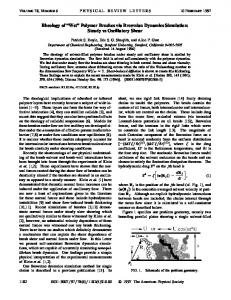
SPT-RDME were generated using the SPT-SSA where the propensities are given by Eq. (3) together with Eq. (5); these were used to obtain a histogram of the particle distribution as a function of time. The mean-field theory (SPT-mfa) is in this case given by Eq. (13) with the histogram of the initial particle distribution from BD as initial condition. In order to integrate the mean-field equation, we use a Euler discretization method where we implemented the nontemporal derivatives using centered difference as this yielded an improved numerical stability. The time and space steps used were t = 10−5 and x = 10−2 , respectively. The diffusion coefficient in the absence of excluded volume interactions is set to unity. The time evolution of the BD, SPT-SSA, SPT-mfa and of the pure diffusion equation with no excluded volume (labeled as “Diffusion”) are compared in Fig. 1. Note that the pure diffusion equation is also the mean-field approximation when the linear law p(θ (x,t)) = 1 − θ (x,t) is used rather than SPT (see Sec. III A). BD (solid light blue region) predicts a highly non-Gaussian shape of the distribution of particles which is highly pointed at the origin for short to intermediate times (t < 1) which smoothens to a Gaussian profile for long times (t = 3). The pointed behavior is due to the fact that because of volume exclusion, only particles at the edge of the rectangular function (which approximately defines the initial conditions) can initially diffuse; this is in contrast to the pure diffusion case (dashed black line) where particles at the edge or center of the rectangular function can diffuse equally easily. As time evolves, the highly packed area becomes less and less crowded,

FIG. 1. Comparison of the SPT modified approaches with Brownian dynamics (BD) for a one species system for various times (a) t = 0, (b) t = 0.8, (c) t = 1.0, and (d) t = 3.0. Both the SSA modified using SPT (SPT-SSA) and the associated mean-field theory (SPT-mfa) reproduce well the BD dynamics, in particular the strongly non-Gaussian behavior at short to intermediate times. Note that position i on the x axis denotes the end of voxel i, not the center of voxel i. This convention is used throughout all the plots. The large differences from pure diffusion (dashed lines) indicate the importance of volume exclusion at intermediate times. See text for further details. 052118-5

CLAUDIA CIANCI, STEPHEN SMITH, AND RAMON GRIMA

PHYSICAL REVIEW E 95, 052118 (2017)

quantitatively measured used the Kullback-Leibler divergence shown in Fig. 2.

0.07 SPT Normal Diffusion

0.06

B. Two species case

KL divergence

0.05 0.04 0.03 0.02 0.01 0 0

0.5

1

1.5

2

2.5

3

Time (s)

FIG. 2. Quantitative measure of the difference between the SPTSSA and BD (lower blue line), and the pure diffusion and BD (upper red line) using the Kullback-Leibler (KL) divergence. Parameters as in Fig. 1. Note the accuracy of the SPT-SSA is reflected in a small KL divergence at all times. The error in the pure diffusion estimate is maximum at intermediate times when the non-Gaussian behavior is most evident.

allowing those particles to move as well hence leading to the Gaussian behavior at long times. Impressively both the SPT-SSA (blue dots) and the SPT-mfa (continuous blue line) are in good agreement with BD at all times; in particular, they reproduce the strong deviations from a Gaussian profile at short to intermediate times. The difference between the methods is

Next, we test the accuracy of our SPT-SSA and mean-field theory versus BD for a two species scenario. The setup is as follows. We consider a setup in which the 3D space in BD is of length 258, width 1, and height 1. Reflecting boundary conditions are enforced. The radius of the two types of particles are 1/14 and 1/28. Initially, 343 particles of the larger radius are packed (on a cubic lattice) in the region 128.5  x  129.5 and 2744 particles of the smaller radius are packed in a region 1×1×1 centered on the position 129.5  x  130.5. The volume occupancy in each of these two regions is 52%. The setup can be approximated by the onedimensional SPT-RDME and its mean-field approximation with unit length voxels as for the previous case. Samples of the process underlying the SPT-RDME were generated using the SPT-SSA where the propensities are given by Eq. (3) together with Eq. (4); these were used to obtain a histogram of the particle distribution. The mean-field theory (SPT-mfa) is in this case given by Eq. (12) with a histogram of the particle concentration (calculated at 0.1 space intervals) taken as the initial condition. The size of time and space steps for BD and the discretization of the mean-field theory PDE are the same as for the one species case. The diffusion coefficient of each species in the absence of volume exclusion, i.e., Di is taken to be unity. In Fig. 3, we display the time evolution of the distribution of the two species according to the various methods, with red denoting the larger species and blue the smaller one.

FIG. 3. Comparison of the SPT modified approaches with Brownian dynamics (BD) for a two species system for various times (a) t = 0, (b) t = 0.1, (c) t = 0.4, and (d) t = 3.0. Red (dark gray) denotes the species with the larger radius and blue (light gray) the smaller sized species. Both the SSA modified using SPT (SPT-SSA) and the associated mean-field theory (SPT-mfa) reproduce well the BD dynamics, in particular, the strongly non-Gaussian behavior in the central spatial region where the two types of particles interact strongly. The large differences from pure diffusion (dashed lines) indicate the importance of volume exclusion at all times. See text for further details. 052118-6

CAPTURING BROWNIAN DYNAMICS WITH AN ON- . . .

PHYSICAL REVIEW E 95, 052118 (2017)

For comparison we also plot the solution of the conventional diffusion equation (no volume exclusion). It is possible to observe that the “external” tails of the BD distribution are actually diffusing almost as much as normal diffusion while the “internal” tails are spreading much slower compared to normal diffusion. This is clearly due to significant volume exclusion induced by particle interaction between the two species in the central region. In particular, according to the theory of Sec. III B the larger species (red) will exhibit a lower diffusion coefficient for positions to the right of the initial central peak compared to the diffusion coefficient on the opposite side of the peak; this effect is further exacerbated by a drift velocity to the left due to the increasing concentration gradient of the smaller species (blue) on the right side of the central peak of the larger species. These effects lead to a highly asymmetrical (and non-Gaussian) shape of the two particle distributions which is distinct from the symmetrical (and non-Gaussian) distribution for one species. Note also that the smaller (blue) particles can be seen moving to the left, whereas the larger (red) particles are not moving right; this makes sense since it is easier for the small particles to permeate the space between large particles than vice versa. Both the SPT-SSA and its mean-field approximation do a very good job of reproducing the BD data at all times, thus verifying the accuracy of the modified RDME for describing heterogeneous systems. V. SUMMARY AND CONCLUSION

In this paper, we presented an effective rescaling of the propensities of the RDME such that we obtain a stochastic spatial description which takes into account volume exclusion due to the finite size of particles and which is applicable to a mixture of particles of different sizes. This is in contrast to the conventional RDME which considers only point particles and to recent modified versions of the RDME [15,17,18,28] which consider volume exclusion but implicitly assume all particles are of the same size. An alternative description to the RDME is provided by the lattice-Boltzmann method. This has recently also been modified using SPT [32] to describe the diffusion of hard disks in a plane; the advantage of our method over the latter is that it provides a three-dimensional description, that it can be used to obtain mean-field equations and that it agrees very well with lattice-free BD simulations. There are three main assumptions in the SPT-RDME: (i) that the diffusion process from one region of space to a neighboring one in BD can be well approximated by a hopping (Markovian) process between two voxels; (ii) the rate of this hopping process is proportional to the probability that a random positioning of the tracer particle will not intersect with any of the particles in the neighboring voxel; (iii) the latter probability is accurately given by SPT. The first assumption is common to the RDME and naturally stems from the artificial discretization of space, hence unavoidable. The second assumption is the natural and probably the simplest choice albeit not the only one. A more accurate choice would be a rate which is inversely proportional to the mean of the first exit time distribution of the tracer. However, it is unclear how to efficiently compute such a quantity for the case of many particles of arbitrary sizes (see [33] for a recent work

in this direction) and, hence, we abandon it in favor of the simpler choice mentioned above. The third assumption is at the heart of our algorithm and indeed it is what foremostly distinguishes it from existing algorithms. SPT takes into account the nontrivial statistical correlations between particle positions (due to volume exclusion) whereas other algorithms do not. For example, in [17,18] the probability that a random positioning of the tracer particle will not intersect with any of the particles in the neighboring voxel is set equal to one minus the fraction of voxel space physically occupied by particles; this overestimates the true probability since there are points of free space between spherical particles which cannot be accessed by a tracer particle due to its finite size. SPT is a more accurate alternative as shown in Appendix A. Also, although in this article we have made use of SPT for a mixture of hard-sphere particles, SPT has also been derived for mixtures of hard convex particles such as right circular cylinders and ellipsoids of rotation [34,35]. Hence, more generally the SPT-RDME and mean-field theory can be used to describe the diffusion of mixtures of hard convex particles which further enhances the applicability and realism of the presented modeling framework. Our comparisons of BD and the SPT-RDME show that the latter is in good agreement with the former, albeit the stochastic simulations take a fraction of the computational time of BD. The mean-field theory obtained as an approximation of the SPT-RDME also does remarkably well, as well as leading to closed-form expressions for the instantaneous and space-dependent diffusion and drift coefficients as a function of particle sizes and local particle numbers. The next clear (and nontrivial) step is to introduce reactions in the RDME and to scale the propensities according to take into account volume exclusion; this will lead to an accurate stochastic description of reaction-diffusion processes between hard-sphere molecules.

ACKNOWLEDGMENT

This work was supported by a Leverhulme grant award to R.G. (Grant No. RPG-2013-171) and a BBSRC EASTBIO PhD studentship to S.S.

APPENDIX A: ACCURACY OF SPT TESTED BY MONTE CARLO SIMULATIONS

In Figs. 4 and 5, we report the results of testing the accuracy of SPT for the single and two particle species cases, respectively. The SPT equations (4) and (5) for multiple and one species, respectively, are compared with the available volume computed from Monte Carlo simulations (see captions for details). We also plot on the same graphs, the prediction of the linear theory which has been used in a number of previous studies [17,18]. Note that the linear theory grossly overestimates the available volume calculated using Monte Carlo simulations, whereas SPT gives an excellent approximation. In Fig. 6, we test the accuracy of SPT as a function of

, the ratio of the particle radius, and the box length for the single particle case. Monte Carlo simulations show that the

052118-7

CLAUDIA CIANCI, STEPHEN SMITH, AND RAMON GRIMA

SPT 1Monte Carlo

0.8

0.8 0.6

0.4

0.2

0.6

0.4

0.2

0

0 0

0.05

0.1

0.15

0.2

0.25

0.3

0.35

0.03

Proportion of occupied volume

FIG. 4. Accuracy of SPT vs linear theory for the single particle case. The SPT equation (5) excellently agrees with the proportion of available volume computed from Monte Carlo simulations. The latter involves calculating the fraction of time that a randomly allocated particle location does not intersect with any of the particles in a random mixture of particles in a cubic box of unit volume. The radius of all particles is 1/20. The proportion of occupied volume is increased through the particle numbers. See text for discussion.

1

Proportion of available volume

SPT 1Monte Carlo

1

Available volume

Proportion of available volume

1

PHYSICAL REVIEW E 95, 052118 (2017)

SPT 1Monte Carlo

0.8

0.6

0.4

0.1

0.3

FIG. 6. Accuracy of SPT as a function of , the ratio of the particle radius, and the box length for the single particle case. The occupied volume fraction is fixed to φ = 0.2. Monte Carlo simulations show that the accuracy of SPT equation (5) is excellent for < 0.2. See text for discussion.

accuracy of SPT is excellent for < 0.2. The large error bar for = 0.2 comes about because when there are only a few large particles, the position of each particle seriously affects the outcome of the Monte Carlo simulations (e.g., one large particle in the middle of the box excludes a lot more volume than one in the corner) so there is a big variability between independent simulations. For = 0.33, almost every attempt to place a particle is rejected, so all Monte Carlo simulations give a result very close to 0, hence the almost invisible error bar. Hence, it is preferable to choose the voxel size to be at least five times larger than the radius of the largest particle; this has been followed for simulations reported in previous figures. APPENDIX B: BROWNIAN DYNAMICS ALGORITHM

0.2

0 0

0.1

0.2

0.3

0.4

0.5

Proportion of occupied volume

FIG. 5. Accuracy of SPT vs linear theory for a two species particle case. The SPT equation (4) excellently agrees with the proportion of available volume computed from Monte Carlo simulations. The latter involves calculating the fraction of time that a randomly allocated position of a particle of species 1 does not intersect with any of the particles in a random mixture of particles in a cubic box of unit volume. The radius of species 1 is 0.02 and of species 2 is 0.05. The proportion of occupied volume is increased through the particle numbers. See text for discussion.

The Brownian dynamics algorithm used in this article is the Cichocki-Hinsen algorithm [3,31], summarized below for the case of N particles with diffusion coefficient D and time step δt: (1) Assign each particle an index 1, . . . ,N and place all N particles at their initial positions. Set time t = √ 0. (2) For i = 1, . . . ,N pick 3 normal(0, 2Dδt) random numbers: the potential new position for particle i is the random numbers added to the current position. If this new position would cause i to intersect with another particle or a boundary, keep the particle in its current position, otherwise move it to the new position. (3) Update t to t + δt. Return to step 2 and repeat until sufficient time has elapsed.

052118-8

CAPTURING BROWNIAN DYNAMICS WITH AN ON- . . .

PHYSICAL REVIEW E 95, 052118 (2017)

[1] J. D. Murray, Mathematical Biology. II. Spatial Models and Biomedical Applications, Interdisciplinary Applied Mathematics, Vol. 18 (Springer, New York, 2001). [2] R. Grima and S. Schnell, Essays Biochem. 45, 41 (2008). [3] B. Cichocki and K. Hinsen, Phys. A (Amsterdam) 166, 473 (1990). [4] S. S. Andrews and D. Bray, Phys. Biol. 1, 137 (2004). [5] J. Lipková, K. C. Zygalakis, S. J. Chapman, and R. Erban, SIAM J Appl. Math. 71, 714 (2011). [6] F. Baras and M. M. Mansour, Phys. Rev. E 54, 6139 (1996). [7] J. Hattne, D. Fange, and J. Elf, Bioinformatics 21, 2923 (2005). [8] A. B. Stundzia and C. J. Lumsden, J. Comput. Phys. 127, 196 (1996). [9] D. Bernstein, Phys. Rev. E 71, 041103 (2005). [10] S. B. Zimmerman and S. O. Trach, J. Mol. Biol. 222, 599 (1991). [11] R. J. Ellis, Trends Biochem. Sci. 26, 597 (2001). [12] R. Grima, J. Chem. Phys. 132, 185102 (2010). [13] D. T. Gillespie, S. Lampoudi, and L. R. Petzold, J. Chem. Phys. 126, 034302 (2007). [14] R. Grima and S. Schnell, Biophys. Chem. 124, 1 (2006). [15] C. Cianci, S. Smith, and R. Grima, J. Chem. Phys. 144, 084101 (2016). [16] M. J. Saxton, Biophys. J. 66, 394 (1994). [17] D. Fanelli and A. J. McKane, Phys. Rev. E 82, 021113 (2010). [18] P. R. Taylor, C. A. Yates, M. J. Simpson, and R. E. Baker, Phys. Rev. E 92, 040701(R) (2015). [19] L. Meinecke and M. Eriksson, arXiv:1604.06660.

[20] M. Bruna and S. J. Chapman, Phys. Rev. E 85, 011103 (2012). [21] M. Bruna and S. J. Chapman, J. Chem. Phys. 137, 204116 (2012). [22] D. V. Nicolau and K. Burrage, Comput. Math. Applicat. 55, 1007 (2008). [23] E. Roberts, J. E. Stone, and Z. Luthey-Schulten, J. Comput. Chem. 34, 245 (2013). [24] S. B. Zimmerman and A. P. Minton, Annu. Rev. Biophys. Biomol. Struct. 22, 27 (1993). [25] H. Reiss, H. Frisch, and J. Lebowitz, J. Chem. Phys. 31, 369 (1959). [26] N. G. Van Kampen and W. P. Reinhardt, Stochastic Processes in Physics and Chemistry (North-Holland, Amsterdam, 1983). [27] T. Marquez-Lago, A. Leier, and K. Burrage, IET Syst. Biol. 6, 134 (2012). [28] M. Galanti, D. Fanelli, A. Maritan, and F. Piazza, Europhys. Lett. 107, 20006 (2014). [29] R. Grima and T. J. Newman, Phys. Rev. E 70, 036703 (2004). [30] C. J. Penington, B. D. Hughes, and K. A. Landman, Phys. Rev. E 84, 041120 (2011). [31] S. Smith and R. Grima, J. Chem. Phys. 146, 024105 (2017). [32] L. Angeles-Martinez and C. Theodoropoulos, BMC Bioinf. 16, 353 (2015). [33] L. Meinecke, arXiv:1603.05605. [34] R. Gibbons, Mol. Phys. 18, 809 (1970). [35] A. P. Minton, Biopolymers 20, 2093 (1981).

052118-9