Capturing Data in the Presence of Noise for Artificial Intelligence

Capturing Data in the Presence of Noise for Artificial Intelligence Systems Aidan Breen, Colm O’Riordan Department of Information Technology, National University of Ireland, Galway {a.breen2,colm.oriordan}@nuigalway.ie

Abstract. In this paper we present the results of a number of experiments testing various methods to rank and sort data in the presence of noise. We model different forms of noise which are intended to simulate output from potentially unreliable sources such as estimated fitness functions, physical sensors, or the results of a study with human subjects. We conclude that while the optimal algorithm in any situation is dependant on the expected noise pattern and the requirements of a specific application, ground truth data can be obtained in most circumstances with a predictable accuracy.

1

Introduction

Gathering information from the real world is inherently noisy. Whether a system relies on sensor data prone to signal fluctuations, destructive sampling which may degrade over time, network data which is constantly changing, or human input which may be outright malicious, there is always some noise present. Artificially intelligent (AI) systems face these challenges more than most, attempting to mimic biological reasoning without the advantage of a biological brain to fill in perceptual blanks.

1.1

Contribution

This work is part of an overall project to illicit correct rankings of items in the presence of noise. We outline a number of potential noise patterns aiming to simulate various real world scenarios. Using the sorting of arrays as a test bed, we compare a number of common approaches to this problem in the presence of different noise patterns. While this contribution is not strictly focused on AI, it is core to many subtopics in the area requiring ground truth data including reasoning systems, genetic algorithms, human computer interaction, knowledge representation, opinion mining, perceptually guided action, recommender systems and sentiment analysis.

2

Related Work

Sorting an array of items is a fundamental task in computer science and many approaches are used. However, introducing noise adds a number of challenges more resembling a tournament ranking challenge whereby values become players and comparisons become matches where the result is not certain. A number of common tournament ranking algorithms exist such as the round robin where each player plays every other player, the knockout tournament where only winning players continue within the tournament, and the Swiss style tournament [1]. A Swiss tournament1 aims to efficiently determine the winner of a tournament using the smallest possible number of matches at the expense of the accuracy of the ranking mid-ranged players. The Swiss tournament is commonly used today for chess and trading card game tournaments where all players in the tournament play the same number of matches [5]. Braverman et al. [2] have studied the ordering of items in the presence of noise. However, they take a theoretical approach to the problem, focusing on a ‘noisy order’ also known as Mallow’s model, and noisy comparisons. In their paper they present ‘polynomial time algorithms for solving both problems with high probability’. While their work on noisy comparisons is related to the work presented in this paper, they provide no empirical results. Furthermore, the omission of implementation details prevented the comparison of their proposed algorithms with the algorithms presented in this paper. Considering a tournament as a directed graph, the minimum feedback arc set (FAS) problem is a related challenge concerned with discovering the minimum number of arcs required to be removed to obtain an acyclic graph. An acyclic graph enables a full, distinct ranking of all nodes on the graph, or players in the tournament. This problem is NP-complete [6]. Recent work by Braverman [2], Kenyon-Mathieo and Schudy [7] and Wauthier [9] explores this area and propose possible approximation approaches. However, the FAS problem focuses mainly on a fair ranking after a large number of arcs have been created, which is not always possible. In many cases, we are limited in the number of samples made, such as in psychological studies or with destructive sampling. Recent work by Breen et al. [3] explores the notion of ranking subjective human preferences, an extremely noisy input, with the minimum number of samples. In this case, samples are limited due to human fatigue. A graph based ranking algorithm is proposed which aims to reduce the number of questions asked of the subject while addressing a number of other methodological issues. 1

A Swiss style tournament begins by randomly pairing competitors. After each round, competitors are given a score — typically 3 for a win, 1 for a draw, 0 for a loss — and paired again but only with competitors with the same, or similar score. The tournament continues until a clear winner is decided. Assuming no draws, a clear winner is decided in the same number of rounds as a knockout tournament, which is the binary logarithm of the number of players rounded up. This reduces the number of comparisons required to finish the tournament but does not produce a full ranking of other players who have not won (or lost) every game.

3

Methods

Eight tournament ranking and sorting algorithms were tested using four noise patterns. A control experiment was conducted without any noise present. The noise patterns are described in detail in section 4. Before the experiments were carried out, a tuning phase was carried out to ensure each noise pattern introduced a similar level of noise to each execution of an algorithm. The details of this tuning phase are outlined in section 3.2 below. A set of 50 randomly ordered arrays of 500 unique integer elements were generated. Each algorithm was executed with each noise pattern to sort all 50 arrays. Each algorithm was implemented with an abstract comparison operator enabling noise to be introduced without altering the implementation of the algorithm. Each algorithm was altered to store the number of times the comparison operator was used while sorting an array. After each array was sorted, it was compared to a correctly sorted array of the same elements and an inaccuracy measure was calculated. Inaccuracy values are normalized and scaled as described in section 3.4 below. 3.1

Noise Patterns

The work in this paper focuses on noisy comparisons. That is, for any ranking or sorting algorithm, a comparison must be made between two elements. If this comparison is not always guaranteed to return the same value given the same two elements, it is said to be noisy. With this is mind, the following sections describe the noise patterns used. Control: The control pattern represents no noise. Every comparison produces the correct result. Percent Noise: This noise pattern introduces a random variance to the values being compared. For any array of values and an input parameter of x percent, each value may be varied by at maximum x percent of the range between the highest and lowest values in the array. For example, for an array of 500 elements, 1 to 500, and a percent parameter of 15, any value being compared may vary by plus or minus 15% of 500 (75). This has the effect of producing unreliable comparisons for elements that are similar in value, and reliable comparisons for elements that are very dissimilar in value. For example, the comparison 110 < 120 should typically be true. With Percent noise applied however, we may actually observe the result of the comparison (110 ± 75) < (120 ± 75) which could be 170 < 103, which is of course false. On the other hand, 30 < 400 will always produce the correct result as the difference of the values is larger than the sum of any potential noise. This noise pattern simulates the effects of reading a signal from a sensor with a random voltage variance.

Flip Noise: This noise pattern represents the comparison operator producing an incorrect result — regardless of the values being compared — with a specific probability. It is similar to the previous pattern in that it introduces random noise to the system. However, this pattern is not sensitive to the actual values being compared, as Percent Noise would be. This noise pattern simulates a human participant who may give the wrong answer to a question through error, or a system where the answer is corrupted through transmission. This type of noise pattern is similar to the ‘noisy comparisons’ used by Braverman et al. [2]. Increasing Noise: This noise pattern also represents the comparison operator producing an incorrect result with a certain probability, similar to Flip Noise above. However, the probability of an incorrect result increases with each comparison made. This simulates destructive sampling or, a human participant becoming more fatigued over time, which will increase the probability of incorrect responses over time. Again, the noise in this pattern is not sensitive to the actual values being compared in contrast to Percent Noise. Tail Noise: This noise pattern, similar to Percent Noise, introduces a random variation of the values being compared. However, in this implementation, the variation of the values is dependant on how large those values are. The lowest value will be subject to no noise, and the highest value will be subject to the maximum level of noise, with noise levels distributed linearly across the values in-between. This noise pattern simulates the output of a fitness function in a genetic algorithm where highly fit individuals may have a far more consistent performance versus less fit individuals. Similarly, within a sporting tournament, highly ranked competitors who maintain a relatively steady performance between matches versus lower ranked competitors who may have varying performance between matches. 3.2

Tuning Noise

We estimate the noise in a system with the Noise Value function, the ratio of false comparisons to true comparisons. A true comparison produces the result we would expect in the absence of noise. We consider n(1) < n(2) = true to be a true comparison, where the function n applies noise to the values 1 and 2. A false comparison produces a result contrary to what we would expect in the absence of noise, and thus we consider n(1) < n(2) = f alse to be a false comparison. With this approach, the input parameters of each noise pattern were tuned resulting in a similar Noise Value for each pattern. 3.3

Algorithms

The results below show the performance of 8 algorithms. Bubble sort (BBL), Insertion sort (INS) and Quick sort (QCK) were chosen as standard sorting

algorithms1 . Round robin (RBN) and Swiss tournament (SWS) were chosen as two tournament ranking algorithms [1]. The graph based ranking algorithm (Graph Sort) proposed by Breen et al. [3] was used with three tie breaking strategies: Random tie breaking (GSR), highest rank tie breaking (GSH) and lowest rank tie breaking (GSL). Details of the Graph Sort algorithm may be found in the appendix. The algorithms selected were chosen to display a variety of approaches and complexities. A summary of the algorithms used is shown in Table 1. Table 1. Tournament Ranking and Sorting Algorithms Algorithm title

Abbreviation Average Complexity

Graphsort - Random tie breaking Graphsort - High tie breaking Graphsort - Low tie breaking Bubble Sort Insertion Sort Quick Sort Swiss Tournament* Round Robin Tournament

GSR GSH GSL BBL INS QCK SWS RBN

nlog(n) nlog(n) nlog(n) n2 n2 nlog(n) log(n) n2

*The Swiss Tournament only achieves a partial ordering.

3.4

Inaccuracy Measure

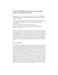
We compare algorithms by an inaccuracy measure based on Spearman’s footrule [4], a measure of the similarity of two arrays of the same elements. Spearman’s footrule was selected as it was quite straightforward to implement, provided a relatively good measure of accuracy and was not computationally expensive. Additionally, Spearman’s footrule was selected over Kendall’s Tau, a similar ranking similarity metric, as it takes into consideration the actual distance between ranked elements. This is an important factor when we attempt to compare algorithms with partially sorted elements. The footrule is calculated as the sum of the absolute difference of position between the elements of the two arrays. The footrule value, f , is calculated for the output of an algorithm and a fully sorted array. This value is non-linear, as demonstrated in Figure 1 and so requires some normalization to produce a linear value and thus make fair comparisons. We modelled the increase in footrule as random values are swapped in an array. A function is easily fitted to the average footrule for 500 arrays which can then be used to estimate the number of swaps, or the inaccuracy, a given footrule represents. This normalization function, solved 1

See [8], pages 106-109, 80-82 and 113-117 respectively

for number of swapped values, S, is S = clog2



b  a−f

where a = 83761.92, b = 83754.69 and c = 178.8318. Finally, the inaccuracy is scaled to plot both the number of comparisons made and the inaccuracy on the same graph.

·104

Footrule (f ) Vs. Swapped values

8

Footrule (f )

6

4

2

0 0

200

400

600

800

1,000

Number of swapped values Fig. 1. Footrule increases non-linearly with random values swapped.

4

Results and Discussion

We now present the results of our experiments. We include some brief analysis of each experiment within the relevant sections below in order to easily delineate the various results for the convenience of the reader. Further discussion and analysis of each algorithm is presented in Section 5 below. Figures 2 and 3 display the average inaccuracy measure and the average number of comparisons made. Error bars display the standard deviation. 4.1

Experiment 1: Control

The control experiment demonstrates the baseline average number of comparisons for each algorithm in Figure 2. We see RBN takes the most number of

Experiment 1: Control

·105

Inaccuracy Comparisons

3

2

1

B

N

S R

SW

S

C K Q

IN

L B B

SL G

SH G

G

SR

0

Ranking Algorithms Fig. 2. Inaccuracy and comparisons for each ranking algorithm under normal conditions. Inaccuracy here is the average normalized footrule value. Comparisons is the average number of comparisons made between two elements in an array for each algorithm over the course of a run.

comparisons, followed by BBL. GSH, GSL and INS perform similarly with the high and low rank tie breaking strategies operating in a similar fashion to INS. With the highest performance here we see GSR, QCK and SWS. SWS produces a partial ordering, with a low number of comparisons as expected, resulting in the only inaccuracy above 0. The aim of this algorithm is to identify the strongest competitor in a tournament in the minimum number of matches, while allowing the other competitors to continue competing against competitors of a similar quality to build experience. A side effect of this approach is that the weakest competitors are also identified. 4.2

Experiment 2: Percent Noise

As shown in Figure 3, Experiment 2, in terms of the number of comparisons needed to reach a partial ranking, RBN and BBL have a very poor performance. A by-product of the large number of comparisons is that the partial ranking produced by both algorithms is much closer to the correct ranking. This is expected as larger numbers of comparisons may reduce the effects of perturbing the data according to a randomly distributed noise pattern. The performance of the other algorithms is generally much better, with less extreme variation. INS, GSL and GSH occupy the middle range with more comparisons and a larger footrule than the higher performing QCK, SWS and GSR. In terms of the number of comparisons, GSR is capable of achieving a partial ranking with the best performance. However, this is at the expense of accuracy where QCK and SWS have the advantage.

G

G

G

B L IN S Q C K SW S R B N

0 B

0

SL

1

SH

1

G

2

SR

2

SL B B L IN S Q C K SW S R B N

3

SH

3

SR

Experiment 5: Tail noise

·105

G

Experiment 4: Increasing noise ·105

G

L IN S Q C K SW S R B N

G

G

G

B

Ranking Algorithms

Ranking Algorithms

Ranking Algorithms

B B

0 SL

0

SH

1

SR

1

B L IN S Q C K SW S R B N

2

SL

2

SH

3

SR

3

G

Experiment 3: Flip noise

·105

G

Experiment 2: Percent noise

G

·105

Ranking Algorithms Inaccuracy Comparisons

Fig. 3. Inaccuracy and comparisons for each ranking algorithm subjected to various noise patterns. Inaccuracy here is the average normalized footrule value. Comparisons is the average number of comparisons made between two elements in an array for each algorithm over the course of a run.

4.3

Experiment 3: Flip Noise

The results of this experiment, shown in Experiment 3, Figure 3, are similar to those generated using Percent Noise: RBN and BBL requiring the most comparisons to produce relatively accurate partial rankings, and GSR, QCK and SWS producing rankings with much fewer comparisons at the expense of accuracy. This is perhaps unsurprising due to the similarities between the two noise patterns. However, there are some variations that may be a result of the lack of sensitivity to the actual values being compared. QCK was relatively unaffected by the change in noise in terms of comparisons made, but suffered greatly in terms of accuracy with an increase in footrule (f ) of 82.587% relative to experiment 2. This is easily justified as the divide and conquer nature of quick sort would lead to large portions of the result being out of place, even if these out of place portions were independently partially sorted. BBL seems to also have suffered greatly in terms of accuracy with a 356.956% increase in f relative to experiment 2. Again, this is because of BBL attempts to bubble each element into place and one incorrect comparison — which can now occur at any point, rather than close to the correct point in the previous noise pattern — can result in an element being placed incorrectly. One incorrect placement like this may then have a further influence on subsequent elements. GSR actually sees an increase in performance here with the number of comparisons decreasing by 20.553% relative to Experiment 2. Interestingly, this increase in performance does not come with a large decrease in accuracy, with f increasing by only 6.067% relative to Experiment 2. 4.4

Experiment 4: Increasing Noise

The results of this experiment are displayed in Experiment 4, Figure 3. BBL sees a large decrease in accuracy relative to Experiment 2 which is most likely due to a similar effect seen with previous noise patterns, where one out of place element may have knock-on effects for further elements. RBN also sees a drastic decrease in accuracy. This decrease, together with the decrease in accuracy we observe with BBL is likely exaggerated due to the increase of noise over time. Both RBN and BBL require the largest number of comparisons which will result in a much greater amount of noise being introduced. GSL, GSH and INS perform similarly with slightly lower numbers of comparisons and slightly decreased accuracy than Experiment 2. SWS remains relatively unaffected with a slight increase of f by 15.851% relative to Experiment 2. This reflects how the algorithm begins by pairing up similarly ranked values, which should achieve a good partial sorting quickly before the noise value increases resulting in values only slightly out of place. GSR shows an increase of f by 28.026% relative to Experiment 2, but as with previous experiments, this increase in accuracy requires an increase in the number of comparisons by 226.774%. While the increase in comparisons may

seem rather large, it should be noted that this remains the lowest number of comparisons of any algorithm in this experiment. Finally, QCK shows the best accuracy and the third lowest number of comparisons — greater than GSR and SWS by 120.733% and 110.036% respectively. Compared to experiment 2, QKC also shows a marked decrease in inaccuracy.

4.5

Experiment 5: Tail Noise

The results of this experiment are displayed in Experiment 5, Figure 3. BBL handles this noise pattern relatively well compared to other noise patterns, performing similarly to the control experiment with a low inaccuracy but high number of comparisons. RBN also achieves a low inaccuracy, but again is the worst algorithm with the greatest number of comparisons. INS, GSH and GSL once again perform similarly, more accurately than Experiment 2 — 29.208%, 29.579%, 29.955% respectively — but with significantly more comparisons — 149.207%, 137.479%, 141.228% respectively. SWS continues to perform well in terms of accuracy but is outperformed on number of comparisons by both QCK and GSR. QCK, performing exceptionally well here with a very strong accuracy and very low number of comparisons. GSR achieves the lowest number of comparisons of all algorithms but with the worst accuracy.

5

Further Discussion

For psychological studies, where human fatigue is a major issue or where destructive sampling techniques are used, the absolute minimum number of samples and a relatively high level of inaccuracy is acceptable. In this scenario, GSR may be preferable. For applications where the number of samples taken, or comparisons made are not a limiting factor, taking as many samples as possible using an approach like RBN is preferable. In a more general scenario where the noise pattern is not predictable or is unknown and a higher accuracy is required, SWS or QCK provide a very predictable accuracy performance with a relatively low number of samples required.

5.1

Algorithm Performance

We now discuss the performance of each algorithm under various noise patterns. In the interest of clarity and to avoid repetition, some similarly performing algorithms have been grouped together.

GSR. GSR performs well across all noise patterns with a low number of comparisons. Indeed GSR actually achieves a lower number of comparisons in the presence of noise than in the control experiment. With the exception of the control, GSR achieves the lowest number of comparisons of any algorithm for each noise pattern. GSR also achieves higher accuracy with some noise patterns, notably handling Increasing Noise quite well. Considering the intended purpose of this noise pattern is to mimic human fatigue and the intended purpose of GSR is to handle this particular circumstance, this is a positive result. GSH, GSL and INS. GSH and GSL perform similarly to each other across all experiments, which suggests that the impact of breaking higher ties versus breaking lower ties is negligible. GSH and GSL also perform strikingly similarly to INS, which may suggest that these algorithms may be slight variations of a generalized sorting pattern. GSH and GSL also perform worse than GSR in every experiment, both in terms of the number of comparisons and accuracy, with the exception of Tail Noise, where GSH, GSL and INS outperform GSR in accuracy. BBL and RBN. BBL and RBN consistently display the largest number of comparisons. This is expected due to the average case complexity of both algorithms. While the performance of these algorithms was perhaps predictable and unnecessary to verify, they do demonstrate a general inverse correlation between the number of comparisons and accuracy achieved. It is plain to see that with the exception of Increasing Noise, a higher accuracy can be obtained using a less efficient algorithm. As mentioned above, this finding may have particular utility in specific circumstances; where a noisy ranking environment is present, making a comparison does not increase the noise, a large number of comparisons is not a drawback and higher accuracy is necessary. SWS. SWS performs incredibly consistently across all noise patterns including the control experiment. This consistency is certainly a major advantage, together with the accuracy it achieves with a low, and predictable number of comparisons. However, in contrast to other algorithms which produce a more homogeneous accuracy distribution, SWS ranks elements with less accuracy towards the center of the array than to either extreme. We suspect the elements ranked closer to the center of the array may be ranked with far less accuracy than the inaccuracy measure used in our results shows. In this respect, SWS cannot be recommended for any application where a homogeneous accuracy is required. QCK. QCK would perhaps be the best choice for experiments 1, 2, 4, and 5 if there was less weight on the number of comparisons made. This algorithm achieves very good accuracy across all noise patterns, with a good number of comparisons for all noise patterns. QCK performs worst in the presence of Flip Noise with a relatively high number of comparisons combined with a lower accuracy than in other experiments.

Future Work We intend to investigate and present the effect of varied levels of noise and how algorithms perform as noise is varied. SWS, GSH and GSL are particularly suited to accurately ranking a subset of values. Their performance may improve when this is specifically measured, and thus we also intend to investigate this.

6

Conclusion

QCK and SWS appear to perform quite well under most circumstances, and may be recommended in circumstances where accuracy is favoured over comparisons made, with SWS particularly suited where consistency is desirable. However they cannot be assumed to be the ideal solution in every scenario. Without any consideration for the number of comparisons, RBN is the ideal solution. Alternatively, in a scenario where reducing the number of comparisons is particularly important, GSR is favourable. The optimal algorithm in any situation will depend on the expected noise pattern, together with the specific application. The accuracy and number of comparison measurements display a rather small standard deviation indicating that the performance of an algorithm under a particular noise pattern is quite predictable. In a scenario where the noise pattern is somewhat predictable, such as human responses in recommender systems or psychological studies, these results may be useful as an indication of the expected relative accuracy of a particular algorithm. Acknowledgement. This research was supported by the Hardiman Scholarship, NUI Galway.

References 1. Appleton, D.R.: May the best man win? JSTOR (1995) 2. Braverman, M., Mossel, E.: Sorting from noisy information. arXiv preprint arXiv:0910.1191 (2009) 3. Breen, A., O’Riordan, C.: Capturing and Ranking Perspectives on the Consonance and Dissonance of Dyads. In: Sound and Music Computing Conference. pp. 125–132. Maynooth (2015) 4. Diaconis, P., Graham, R.L.: Spearman’s footrule as a measure of disarray. Journal of the Royal Statistical Society. Series B (Methodological) pp. 262–268 (1977) 5. Just, T., Burg, D.B.: US Chess Federation’s Official Rules of Chess , McKay. Tech. rep. (2003) 6. Karp, R.M.: Reducibility among combinatorial problems. Springer (1972) 7. Kenyon-Mathieu, C., Schudy, W.: How to rank with few errors. In: Proceedings of the thirty-ninth annual ACM symposium on Theory of computing. pp. 95–103. ACM (2007) 8. Knuth, D.E.: The art of computer programming, volume 3: sorting and searching. Addition Wesley (1973) 9. Wauthier, F.L., Jordan, M.I.: Efficient Ranking from Pairwise Comparisons. Proceedings of the 30th International Conference on Machine Learning 28, 1–9 (2013)

Appendix: Graph Sort Algorithm The Graph Sort algorithm, proposed by Breen et al. [3] is designed to minimize the number of comparisons required to find a complete ranking based upon the use of a directed graph. To sort an array, each element is represented as a node on a graph. Beginning with a fully unconnected graph, all nodes are ranked equally at 0, directed edges are added between nodes based on the tie breaking approach. In this paper we explore three tie breaking approaches: Random tie breaking (GSR), Highest rank tie breaking (GSH) and Lowest rank tie breaking (GSL). After each edge is added to the graph, the rank of each node is recalculated. Given the number of forward reachable nodes from any node n as δnf , the rank R of any node is defined as R(n) = δnf + 1. This process continues until no ties remain, resulting in a complete ranking. Table 2. Common Experiment Parameters Parameter

Value

Array size 500 Arrays for each noise pattern 50 Tuned to noise value 0.9

Table 3. Noise Pattern Parameters Pattern

Description

Control

No noise. Comparisons and values are always correct.

None

Percent noise

Values vary by a percentage of the total range of values.

Value Range (0-500), Percent (15)

Flip noise

Comparison result is inverted with a predefined probability.

Probability (0.105)

Increasing noise Flip noise with an increase in probability of an incorrect result each time a comparison is made. Tail noise

Percent noise with an increase of noise for larger values.

Parameters (values)

Init. Probability (0), Increment (0.0000045)

Value Range (0-500), Percent Range(0-120)