{claus.brenner, monika.sester}@ikg.uni-hannover.de ... These approaches usually start from geometric representations like polygons or lines. From this .... where g subsumes the possibly contradictory, “weak” constraints, whereas f .... (a) Original graph, (b) perfect matching, (c) strongly connected components, (d) collapsed.
CARTOGRAPHIC GENERALIZATION USING PRIMITIVES AND CONSTRAINTS C. Brenner, M. Sester Institute of Cartography and Geoinformatics, University of Hannover, Germany {claus.brenner, monika.sester}@ikg.uni-hannover.de
We propose the use of primitives, containers, and constraints as a computational means for cartographic generalization. Primitives bundle object geometry and internal constraints, as well as a discrete behaviour. Containers are collections of primitives which also exhibit a certain behaviour, such as arranging their children in a linear way or as a regular pattern of rows and columns. Together, they form a hierarchy of containers and primitives which is used to lay out a map. This layout is ultimately determined by putting together all constraint equations, and finding an overall solution which minimizes certain criteria while enforcing strict constraints at the same time. We explore the handling and solution of constraint equation systems by looking into constraint graphs, Gröbner bases, and row reduction of Jacobi matrices.
INTRODUCTION Cartographic generalization has been tackled by many researchers and satisfactory results have been achieved in the past. These approaches usually start from geometric representations like polygons or lines. From this, implicit relationships are discovered, such as parallel and rectangular structures, distances, protrusions, etc., which are to be modified or preserved in the subsequent generalization step. The final outcome is again a description of the objects in terms of their geometry only. This approach has the disadvantage that the implicit information about the structure of the objects and their relationships is derived, used, and discarded immediately after. Thus, a user typically cannot see what structures were discovered, nor can he influence them, except for some general parameter settings. Recently, in cartography methods are being investigated and developed which aim at the recognition of important structures that are needed as a basis for generalization, e.g. parallelism, linear arrangement, clusters (Christophe & Ruas, 2002, Anders & Sester, 2000, Neun et al., 2004). Furthermore, there are approaches which try to separate generalization processes related to different objects in different hierarchical levels, e.g. when defining generalization modules that can be handled independently (Kilpeläinen & Sarjakoski, 1995). A first attempt to explicitly model these structures has been done in the AGENT project, where different hierarchical levels of objects have been specified that can act independently with a specific dedicated behaviour (Lamy et al., 1999). In computer aided design (CAD) research, there have been numerous approaches to construct parts by using predefined primitive objects, which are combined using construction rules, represented as constraints. For example, constraints enforce that planes meet, axes are the same, or dimensions are equal or in a fixed relation to each other. Modeling objects this way does not only allow to reuse parts from a parametric part library, but also has the advantage that the original design intent of the part designer is represented explicitly in terms of those relationships. Applying this approach to cartographic generalization implies that object structures and their relationships are described in an explicit manner. This makes it possible to modify the original description, adding or re-weighting relationships as needed, in order to change the generalization outcome. This leads to a more elaborate description of the objects, however with the benefit of being able to derive fully automatically different generalization levels. Thus, the use of parts and constraints in cartographic generalization goes beyond a ‘single instance’ description: as scale changes, parts and constraints might change or vanish, too, i.e. generalization rules for both parts and constraints have to be available.
CONSTRAINT EQUATIONS A geometric constraint problem consists of a set of geometric primitives and a set of constraints between them. Geometric primitives are e.g. points, lines, or circles. Constraints may be logical, such as incidence, perpendicularity, parallelism, tangency, etc., or metric such as distance, angle, radius, etc. Finding a solution for a given set of constraint equations is equivalent to finding a real solution to the corresponding algebraic equation system.
Constraint equations can usually written as algebraic equations of the form f i ( x ) 0 , where x R n is the parameter vector describing the scene. For example, x can directly contain coefficients describing primitive objects such as points and lines but can also describe “higher level” parameters such as the transformation parameters of a substructure. Putting all the functions f i , 1 i m together, the problem is to find a parameter vector x which satisfies the implicit (and, usually, nonlinear) constraint equation f ( x) 0
(1)
This equation can be either underconstrained, well constrained, or overconstrained, depending on the number of unknowns and constraints. In the latter case, the system has either no solution at all or it is consistently overconstrained, i.e. there are more equations than needed, which are however not independent. As opposed to linear systems, a zero dimensional solution space can still involve a large number of individual solutions x, exponential in the number of equations. Also, the idea that each “independent” equation reduces the “dimension” of the solution space by one is more involved, for example (Cox et al., 1997), given the two nonlinear equations f1 xz 0 and f 2 yz 0 with x ( x, y , z ) T R n , the solution space is the union of the z-axis with the (x,y)-plane, i.e. the union of a one- and twodimensional subspace.
In CAD research, a common problem is as follows: given a sketch of an object, annotated with dimensional information, construct an instance of that object. The sketch gives information about the involved geometric primitives and their relationships, while the annotation gives the dimensions, which together allows to set up the constraint equations. In this case, it is desirable that the system is well constrained or consistently overconstrained. Typically, relationships derived from the sketch or additional user input are used to pick out the individual solution.
(a)
(b)
(c)
Figure 1: Change of a linear row of objects during generalization. (a) Original state, (b) when linearity is not enforced, (c) with linearity enforced.
When generalization problems are written as equation systems, there are usually two equation types present: equations that should be fulfilled “as best as possible”, and constraint equations which must hold. For example, in Figure 1(a), suppose the situation of a linear row of objects was detected. If those objects get “under pressure” by a scale change (illustrated by the two arrows), they will escape as shown in Figure 1(b) if they are forced to keep their distances. However, if an additional linearity constraint is introduced, they are forced to lie on a line, as shown in Figure 1(c), although the goal of keeping the distances cannot be met. For the equation system, this means that there are two equations, !
g ( x ) min , subject to
f ( x) 0 ,
(2)
where g subsumes the possibly contradictory, “weak” constraints, whereas f represents the “hard” constraints. As opposed to the mentioned case in CAD, f will be normally underconstrained (as else the hard constraints would determine the layout completely), whereas g will be often overconstrained (when multiple requirements compete against each other), which leads to a system which is both locally overconstrained and globally well- or underconstrained. The globally underconstrained case is interesting since it leaves room for interactive manipulation of objects which are not fixed by either weak or hard constraints. As f is usually nonlinear, it cannot be solved analytically in general. However, one can try to (i) exploit the special structure of the equations, (ii) exploit the type of the equations, which are often polynomial, or (iii) linearise the equations and solve them iteratively. These cases are briefly discussed in the following section.
ANALYSIS OF CONSTRAINT EQUATIONS Exploiting Structure When a drawing is constructed using compass and ruler, a step-by-step procedure is usually applied. That is, objects are added one-by-one as soon as there are enough constraints which allow to place them unambiguously. (Instead of successively adding single elements, it might also happen that complete “subgroups” have to be constructed separately which are assembled only at the end.) Approaches which exploit this are called constructive constraint solvers. Their goal is to decompose the original constraint system into small, manageable subsystems, solve them, and recombine the solutions to an overall solution. The decomposition should be optimal in such a way that the size of the largest subsystem is minimized. A decomposition-recombination (DR) plan can be made as a preprocessing step before actually starting to solve the equation system. Two major types of DR plans are constraint shape recognition (Owen, 1991, Fudos & Hoffmann, 1997) and generalized maximum matching (Kramer, 1992, Ait-Aoudia et al., 1993), see (Hoffmann et al., 2001) for an overview. In the following, the basic principles of the latter are sketched. Suppose, upon closer examination of (1), it turns out that f 0 consists of the following equations (Ait-Aoudia et al., 1993): f1 ( x1 , x2 ) 0 , f5 ( x3 , x5 , x7 ) 0 ,
f 2 ( x1 , x2 ) 0 , f6 ( x4 , x5 , x6 ) 0 ,
f3 ( x2 , x3 , x4 ) 0 , f 7 ( x6 , x7 ) 0 .
f 4 ( x1 , x3 , x4 ) 0 , (3)
From this, a constraint graph can be derived, which contains a node for each constraint and unknown, and an edge if an unknown appears in a constraint, see Figure 2(a). This bipartite graph G captures structural properties of the equation system. G is said to be structurally well-constrained if there are as many constraint nodes as unknown nodes and for no subset of constraints, there are less unknowns than constraints. If U () returns the set of unknowns for a given set of
equations, i.e. if F { f1 , , f 7 } , then U ( F ) {x1 , , x7 } , then, in the example graph, 7 F U ( F ) , and for any subset F ' F , F ' U ( F ' ) . If for a well constrained graph the property F ' U ( F ' ) holds for any true subset F ' F , the graph is said to be irreducible. Any well constrained graph is either irreducible or contains an irreducible subgraph. One is interested in irreducible subgraphs, since they correspond to smaller size subproblems which are easier to solve. f1
f2
f3
x1
x2
x3
f1
f2
f3
x1
x2
x3
f4
f5
f6
f7
f1
f2
f3
x4
x5
x6
x7
x1
x2
x3
(a) f4
f5
f6
f7
x4
x5
x6
x7
(c)
f4
f5
f6
f7
x4
x5
x6
x7
(b) H11
H12
H13
(d)
Figure 2: Constraint graph for Eq. (3). (a) Original graph, (b) perfect matching, (c) strongly connected components, (d) collapsed graph H.
The irreducible subgraphs of a graph can be computed from a perfect matching (a set of edges where no two distinct edges share a vertex and all vertices are covered, Figure 2(b)) by finding strongly connected components, Figure 2(c). By collapsing the irreducible subgraphs to single nodes, and replacing the edges between them by single, directed edges, a new graph H is obtained, which is acyclic, Figure 2(d). It induces a partial order which can be used to solve the equation system. In the example, H 11 H 11 ( x1 , x 2 ) can be solved first, since it contains two equations f1 , f 2 , dependent on two unknowns x1 , x2 . Then, H 12 H 12 ( H 11 , x3 , x 4 ) can be solved, since there are two equations f 3 , f 4 , which depend on four unknowns, however, x1 , x2 are known already, so x3 , x4 are obtained. Finally, H 13 H 13 ( H 12 , x5 , x6 , x7 ) can be solved using the values for x3 , x4 .
It has to be noted that since G captures only structural properties, there is not always a one-to-one relationship between G and the original equation system E: G can be overconstrained, while E still has a finite (or infinite) set of solutions (in case of consistent overconstraints); G can be underconstrained but E can still have a finite set of solutions (consider
x12 x22 0 over the reals); or G can be well-constrained but E has an infinite set of solutions (when the Jacobian C of f
does not have full rank). If G is not well-constrained, the method above will find subgraphs G1 , G2 , G3 , which are well-, over-, underconstrained, respectively.
Polynomial Equations Constraints between objects can often be expressed using bilinear equations. For example, in the two-dimensional case, with p ( x1 , y1 ) T , q ( x2 , y 2 ) T R 2 denoting points and l ( a1 , b1 , c1 ) T , m ( a 2 , b2 , c2 ) T representing lines in Hesse normal form ax by c 0 , a12 b12 1 0 ,
a1 x1 b1 y1 c1 0 a1 x1 b1 y1 c1 d 0
(4) (5) (6)
a1a2 b1b2 0 a1b2 a2b1 0
(7) (8) (9)
( x1 x2 ) 2 ( y1 y 2 ) 2 d 0
a1a2 b1b2 cos 0, a1b2 a2 b1 sin 0
(10)
are equations for (4) l having a unit length normal vector, (5) p incident l, (6) p having (signed) distance d from l, (7) p having Euclidean distance d from q, (8) l perpendicular m, (9) l parallel m, (10) oriented lines l and m enclosing the fixed angle . (See e.g. (Heuel, 2004) for a more complete list of relationships.) Thus, f from (1) consists of a set of polynomial equations f i ( x ) 0 , for 1 i m . The set of all solutions x which satisfy all those equations is called the affine variety (Cox et al., 1997) V ( f1 , , f m ) , i.e. V ( f1 , , f m ) { x R n : f i ( x ) 0 1 i m} .
The corresponding algebraic object is the ideal I, which is a subset of all polynomials over a field which satisfies (i) 0 I , (ii) f1 , f 2 I f1 f 2 I , (iii) f1 I , h polynomial hf I . I.e., I always contains the zero polynomial, the sum of two polynomials from I is also in I, and the product of a polynomial from I with any polynomial (not necessarily from I) is also in I. Now given the set of polynomials f1 , f m , the set m f1 , f m : hi f i i 1
with hi being arbitrary polynomials over the field is indeed an ideal, the ideal generated by f1 , , f m . Interestingly, it turns out that the variety V ( f1 , , f m ) does not depend on the particular basis functions chosen, but rather only on the ideal generated by them, i.e. V ( f1 , f m ) V ( f1 , , f m ) .
The consequence of this is that if we are given a set of polynomial equations f1 , , f m and are looking for their solution space V ( f1 , , f m ) , we can replace the original set of polynomials by any other set h1 , , hs for which f1 , , f m h1 , hs , i.e. which spans the same ideal.
A particularly useful set is the Gröbner basis of an ideal I, a finite set h1 , , hs for which LT ( h1 ), , LT( hs ) LT( I ) ,
where LT(h) denotes the leading term of the polynomial h under a given monomial order and LT ( I ) is the ideal spanned by all leading terms of I. The Gröbner basis can be systematically obtained from any given set of polynomials using Buchberger’s algorithm. It is the generalization of the familiar row reduction for linear matrices, and in fact it will yield the row reduced form of a matrix if applied to a linear equation system. Gröbner bases can be used to solve polynomial equation systems, since they can successively eliminate variables. That is, as linear equations can be solved using row reduction followed by back substitution, a polynomial equation system can be solved by computing a Gröbner basis h1 , hs , then solving the “last” equation hs 0 , which contains the “last” variables (according to the given monomial order), and successively back substituting and solving hs 1 , hs 2 , …, h1 . Unfortunately, not only the number s of polynomials in the Gröbner basis can be very large, but also the order of the polynomials. It has been shown that the construction of a Gröbner basis from polynomials of degree of at most d can d
involve polynomials of degree proportional to 2 2 , and thus even if a Gröbner basis can be obtained, the polynomials can usually only be solved numerically.
However, Gröbner bases have also the property that the ideal membership problem can be solved using polynomial division. That is, the question if a given polynomial f is member of the ideal I can be answered easily by dividing f by the polynomials h1 , , hs of the Gröbner basis of I. If there is no remainder, f I . For the corresponding varieties, this means that for any solution x V (I ) , also f ( x ) 0 holds. In the context of generalization, this can be used as follows. Given a partially constrained scene, involving variables x and constraints h1 , , hs 1 , the relation to another constraint hs is to be checked – e.g. since it is to be added or removed from the set of constraints. Now this additional constraint can (i) really add information (which is what usually is intended), (ii) be superfluous (since the constraint is actually already enforced by some combination of h1 , , hs 1 ), or (iii) can render the system unsolvable. These cases can be distinguished as hs I h1 , , hs 1 h1 , , hs 1 case (iii), and else case (i) holds.
case (ii),
Altogether, this approach can be used to identify redundant as well as conflicting constraints. However, the caveat is that computing a Gröbner base can take substantial time and space, so that its computation is not feasible in an interactive environment. The question here is if the special nature of the equations involved, such as (4)-(10), can somehow lead to lower time and space bounds.
Linearisation of Equations The linearisation of (2) results in an equation system of the form !
Ax b min , subject to
(11) (12)
Cx d .
where A and C are the design and constraint matrices, respectively (a weight matrix is omitted for clarity). If
in
(11) is the L 2 norm, this can be solved in numerous ways (Lawson & Hanson, 1995), (i) by weighting ~ A ~ b A , b C d
~ ~ with some “large” , and minimizing Ax b using the normal equations
~ ~ ~ ~ A T Ax A T b
(13)
(ii) by introducing Lagrange multipliers k and solving AT A C T x A T b 0 k d C
(14)
or (iii) by an explicit parametrisation of the null space of C: since all solutions to (12) can be parameterized as x C d Ny , where the columns of N span the null space of C and C is the Moore-Penrose pseudoinverse, instead of minimizing (11) over all x, one can minimize A(C d Ny) b with respect to y, which yields (Lawson & Hanson, 1995) x C d (A(I n C C)) (b AC d) .
(15)
A problem arises with (13), since it enforces the constraint equations (12) only to a certain degree, dependent on . As ~ constraint equations might compete against observation equations, has to be set very high, running the risk that A gets poorly conditioned. One can think of situations where the requirement to exactly fulfil the constraints (12) can be relaxed. For example, it might be not so important that a right angle is exact to 8 decimal places. However, C usually also contains incidence relations which must be satisfied in order for subsequent CAD operations, such as Boolean union or intersection, to succeed. Care must also be taken considering the rank of the matrices. Problem (11,12) has only a unique solution if [ AT , C T ] has full rank. If not, solutions based on normal equations and inversion (13), (14) are not suitable, but pseudoinverse (15) or SVD solutions are. As noted earlier, in the context of generalization, scenes are usually underconstrained.
AN EXAMPLE Consider the left polygon in Figure 3(a), which is to be simplified to a four-sided polygon as the result of a generalization operation. In Figure 3(b), only the relevant part of the object is shown. The generalization operation will remove the “intrusion” consisting of points p1 , p2 , p3 and lines l 2 , l3 , while l1 and l 4 are kept and intersected to form the new point p. All the points must lie on their corresponding lines, and the lines must have normal vectors of length one, which yields the following constraints: p1 l1 , l 2 , p2 l2 , l3 , p3 l3 , l 4 , i.e. 6 equations of type (5) plus 2 equations of type (4), for a total of 8 equations. When the generalization operation removes the points and lines, all those constraints will vanish, too. l4
p3 p1 l1
l3 l2
p l1
p2
(a)
l4
(b)
l1
?
l4
(c)
Figure 3: Removing an intrusion as result of generalization. (a) Illustration of the operation, (b) lines and points along the intrusion, (c) the situation when the removed part includes geometric constraints.
However, consider the case in Figure 3(c), where additional constraints hold between the objects which are removed. In addition to the 8 equations from above, there are now three right-angle constraints l1 l 2 , l 2 l3 , l3 l4 . In this simple example, it is easy to see that these three constraints actually force l1 to be perpendicular to l 4 , by the chain l1 l2 l3 l 4 . This means that if the generalization operation takes out the geometry and the constraints as well, the information l1 l 4 will be lost. In the following, it is discussed how this can be detected using the methods from the previous section.
Structural Detection Using the Constraint Graph Figure 4 shows the bipartite constraint graph for the situation in Figure 3(c). There are a total of 8+3=11 constraints as laid out above, unknowns for the points pi ( xi , yi ) T and lines li ( ai , bi , ci ) T , for a total of 18 unknowns (degrees of freedom). As there are only 11 constraints and 18 unknowns, the graph is underconstrained and there is no perfect matching. In order to find out if the constraints impose any condition on l1 and l 4 , we fix them (shown in grey). Now there are still 11 constraints and 12 unknowns, however the structure reveals that the graph is nevertheless overconstrained: it is impossible to match all of the three rectangularity nodes, leaving one of them unmatched (e.g. the rightmost, as shown in Figure 4). Thus, from the constraint graph, it becomes clear that l1 and l 4 are related. Note,
however, that the constraint graph is unable to tell whether the corresponding equation system is solvable or not: if l1 l 4 is enforced by some other equations (e.g. when all angles in the polygon Figure 3(a) are right angles), the unmatched rectangular node is an consistent overconstraint which can be removed. i a1 b1 c1
r x1 y1
i
n
i
a2 b2 c2
r x2 y2
i
n a3 b3 c3
i
r x3 y3
i a4 b4 c4
Figure 4: Bipartite graph representing the objects and constraints of Figure 3(c), with maximum matching shown as bold lines. Upper row: i, r, n are incidence (Eq. 5), rectangularity (Eq. 8), normal vector (Eq. 4) constraints, respectively. Lower row: unknowns for the four lines and three points. Unknowns in grey circles are held fixed.
Detection using Gröbner Bases In order to detect if the 11 equations impose any constraint, all unknowns have to be eliminated except for the unknowns of l1 and l 4 . This can be achieved by specifying the variable order x1 > y1 > …> y3 > a2 > b2 > c2 > a3 > b3 > c3 > a1 > b1 > c1 > a4 > b4 > c4 (with the unknowns of l1 and l 4 being last) and computing a Gröbner basis. With lexicographic monomial ordering, the basis contains 34 terms, {a3 c3 x1 a2 c2 x3 x1 x3 b3c3 y1 b2 c2 y3 y1 y3 , …, -a42+a 42b32+b32 b42 , a1a4 b1b4 } . The last equation is the only one involving unknowns from l1 and l 4 only, and one sees
that a1a4 b1b4 0 is exactly of type (8), l1 l 4 . Thus, the Gröbner basis reveals that there is a constraint indeed, enforced by the constraints of the intrusion, and moreover that it is a rectangularity constraint. In contrast to the structural analysis of the previous subsection, the Gröbner basis will reveal consistent overconstraints. If l1 l 4 by some other constraints, the three equations a1a4 b1b4 0 , a12 b12 1 , a42 b42 1 hold for the situation without the intrusion. This leads to the Gröbner basis B { a12 b42 , a1b1 a4b4 , a1a4 b1b4 , a1 a4 b1b4 a1b42 ,
1 b12 b42 , 1 a 42 b42 } . On the other hand, when the 11 equations from above are combined with these three
equations, and all unknowns except those for l1 and l 4 are eliminated, exactly the same Gröbner basis is obtained. This means that the additional constraint imposed by the equations of the intrusion is not independent; rather, it is a consistent overconstraint. Alternatively, it may be checked that f a1a4 b1b4 , obtained from the analysis of the intrusion constraints, is in the ideal spanned by B, i.e. f B , which is obviously the case since in fact, f B .
Detection using Linearisation A similar result can be obtained if the 11 equations are linearised and all unknowns except the ones for l1 and l8 are eliminated. Suppose the linearisation point is p1 (0,0) T , p 2 (1,0) T , p3 (1,1) T , l1 (1,0,0) T , l 2 (0,1,0) T , l3 (1,0,1) T , l 4 (0,1,1) T , then the Jacobi matrix of the partial derivatives with respect to the variables x1 , y1 , x2 ,
y2 , x3 , y3 , a2 , b2 , c2 , a3 , b3 , c3 , a1 , b1 , c1 , a4 , b4 , c4 (in that order, with variables to be eliminated first) is
ijj jjj jjj jjk 1 0 0 0 0 0 0 0 0 0 0
0 1 0 0 0 0 0 0 0 0 0
0 0 1 0 0 0 0 0 0 0 0
0 0 0 1 0 0 0 0 0 0 0
0 0 0 0 1 0 0 0 0 0 0
0 0 0 0 0 1 0 0 0 0 0
0 0 0 0 0 0 1 0 0 0 0
0 0 0 0 0 0 0 1 0 0 0
0 1 0 1 0 0 0 0 0 0 0
0 0 0 0 0 0 0 0 1 0 0
0 0 0 0 0 0 0 0 0 1 0
0 0 -1 0 -1 0 0 0 0 0 0
0 0 0 0 0 0 0 0 0 0 0
0 -1 0 0 0 0 0 0 0 0 0 0 0 0 0 0 0 1 0 0 0 0 -1 0 0 0 0 1 1 1 0 0 -1 0 0 0 0 0 0 0 0 0 0 0 0 0 0 -1 0 0 1 0 -1 0 0
y z z z z z z z z z z {
after it has been row reduced. Then, from the last line of this matrix, it can be seen that l1 and l 4 are not independent (this is the equivalent to the equation a1a4 b1b4 remaining in the nonlinear case). As in the nonlinear case, one can check if the intrusion changes anything when l1 l 4 is enforced by some other constraints. The three equations (one for l1 l 4 and two for unit normal vectors) lead to the row reduced Jacobi matrix
jijk
0 0 0 0 0 0 0 0 0 0 0 0 1 0 0 0 0 0 0 0 0 0 0 0 0 0 0 0 0 0 0 1 0 -1 0 0 0 0 0 0 0 0 0 0 0 0 0 0 0 0 0 0 1 0
y z z {
which is in fact also the last part of the row reduced Jacobi matrix of the 14 equations. That is, the same result is obtained, no matter if (a) only the three equations are used, describing l1 l 4 and unit normal vectors, or (b) these three equations plus all 11 constraints from the intrusion are used and all variables except the ones for l1 , l 4 are eliminated.
PRIMITIVES AND CONTAINERS From the previous example, it can be seen that tools are available which can discover implicit or contradictory constraints. Constraint graphs show structural dependencies, Gröbner bases reveal dependencies of polynomial equations, and the Jacobi matrix shows similar results for the linearised equations. This can be either used when constraints are inserted manually or after they have been inferred automatically from a given scene. However, up to now, we have considered constraints to be “flat”, i.e. not being tied to some hierarchy. For example, modelling the polygon as shown in Figure 5(a), with all angle constraints being between pairs of successive segments, leads to the constraint graph in Figure 5(b). One angle constraint has been omitted in order to keep it well constrained. If l 2 , l3 are removed, the situation discussed in the previous section is encountered, where the removal of the intrusion leads to the loss of an angle constraint to l1 unless the implicit constraint is uncovered and made explicit (Figure 5(c)). However, the orientation of all the segments in the polygon can also be seen as a higher-level object constraint. Introducing an “object orientation”, all the segments can be tied by constraints to it, as shown in Figure 5(d). Then, the constraint graph (Figure 5(e)) does not expose long dependency chains, and removing parts does not cause implicit angle constraints to be lost, Figure 5(f). 90
90
90
90
90
90
90
90
1 2 3 4 5 6
(b)
(c)
0
(d)
90
1 2 3 4 5 6
(a)
90
90
0
90
0
90
1 2 3 4 5 6
(e)
0
90
0
90
0
90
1 2 3 4 5 6
(f)
Figure 5: A polygon where all angles are fixed, modelled either as angle constraints between successive segments (a,b,c) or dependency on a general orientation (d,e,f).
In order to introduce constraints in a systematic manner, they can be “packaged” into primitives. That is, instead of attempting to set up an object by first specifying the geometry and then introducing all appropriate constraints, it comes “pre-wired” with all constraints automatically established. In fact, primitives are only one part of an object-oriented concept with the following properties: 1. 2. 3. 4.
objects may be primitives, in which case they contain explicit geometry, or they may be containers, which recursively contain other objects, objects exhibit a discrete behaviour: a primitive may generalize its outline polygon by leaving out minor structures; a container may leave out some of its children according to some specified pattern, objects exhibit the ability to place constraints automatically: for example, all the orientation constraints for the segments of a polygon will be inserted automatically, objects offer an interface which allows to connect primitives to containers, or containers to containers.
Part of this concept has been introduced earlier as “weak primitives” in another context (Brenner, 2004). The basic idea behind weak primitives is to provide objects looking like constructive solid geometry (CSG) entities with implicitly enforced properties, however being internally boundary representations with explicitly formulated constraints. This concept has the advantage that it is possible – in contrast to CSG – to relax constraints when needed. Moreover, external
constraints which force objects to meet, be rectangular, have a certain distance, etc. integrate seamlessly with internal constraints in a common constraint framework. Weak primitives are extended here with respect to discrete behaviour. As primitives and containers might undergo a discrete change as result of a generalization operation, constraints must be established automatically. For example, in a linear row of evenly spaced objects, removing one of the objects needs to automatically establish a constraint between the two new neighbours. Figure 6 shows examples of primitive and container objects, examples for their discrete behaviour and internal constraints. Object type
Discrete behaviour examples
Internal constraint examples Angle and distance constraints between polygon parts.
Polygon (primitive)
Linear (container)
Boundary simplification.
Remove single elements.
Centres on a line, front along a line, even spacing, same orientation. Minimum distance to left/right neighbour set up automatically. Even spacing, same orientation. Minimum distance to left/right/up/down neighbour set up automatically.
Regular (container)
Remove rows and/or columns, but not single elements. Keep spacing/spacing ratio. Minimum distance to adjacent objects set up dynamically.
Irregular (container)
Remove single elements, approximate density.
Figure 6: Examples for object types, their discrete behaviour, and typical internal constraints.
CONCLUSIONS In this paper, we have proposed to use primitives, containers, and constraints as a means for cartographic generalization. A primitive bundles geometry, constraints, and discrete behaviour. It is like a CSG primitive, however the boundary is not given implicitly but rather explicitly with additional constraints enforcing regularity, which is termed a “weak CSG primitive”. In addition, discrete behaviour allows a primitive to change its representation and set up modified constraints automatically. Primitives expose an interface, which essentially allows to “connect” them to other objects. There is no difference between internal constraints and external constraints defined by such connections. Usually, primitives will be connected to containers, which do not carry geometry themselves, but rather only by the objects they contain. Just like primitives, containers imply a certain discrete behaviour and expose an interface which can be used to connect them recursively. Determining a map representation of a certain generalization level amounts to finding a solution which optimises a function under a set of constraints. That is, a part of the equations has to hold in a “best possible” way, whereas the other part is required to be exactly fulfilled. For that purpose, we have looked into how constraint equations can be handled and solved. We have explored three major approaches: structurally, using the constraint graph and maximum matchings; nonlinear, limited to polynomial constraints, using Gröbner bases; and linear, using the Jacobi matrix and row reduction. The application of those techniques has been shown for a simple example where an intrusion was removed from a polygon.
ACKNOWLEDGEMENT This work has been supported by a research grant from the VolkswagenStiftung, Germany.
REFERENCES Ait-Aoudia, S., Jegou, R. and Michelucci, D., 1993. Reduction of constraint systems. In: Compugraphics, pp. 83-92. Anders, K.-H., Sester, M., 2000. Parameter-Free Cluster Detection in Spatial Databases and its Application to Typification, International Archives of Photogrammetry, Remote Sensing and Spatial Information Sciences, the Netherlands, 16-23 July 2000, Vol. XXXIII, Part A4 (CD-Rom). Brenner, C., 2004. Modelling 3D Objects Using Weak CSG Primitives , in: `International Archives of Photogrammetry, Remote Sensing and Spatial Information Sciences', Vol. 35, ISPRS, Istanbul, 2004. Christophe, S., and Ruas, A., 2002. Detecting Building Alignments for Generalisation Purposes. International Symposium on Spatial Data Handling (Canada / Ottawa, 2002), pp. 419-432, SDH 2002. Cox, D., Little, J. and O'Shea, D., 1997. Ideals, Varieties, and Algorithms. Springer Verlag New York. Fudos, I. and Hoffmann, C. M., 1997. A graph-constructive approach to solving systems of geometric constraints. ACM Trans. on Graphics 16(2), pp. 179-216. Guibas, L. J., Overmars, M. H. and Robert, J.-M., 1996. The exact fitting problem for points. Comput. Geom. Theory Appl. 6, pp. 215-230. Heuel, S., 2004. Uncertain Projective Geometry : Statistical Reasoning for Polyhedral Object Reconstruction. Springer LNCS. Hoffmann, C. M., Lomonosov, A. and Sitharam, M., 2001. Decomposition plans for geometric constraint systems, part I: Performance measures for CAD. J. Symbolic Computation 31, pp. 367-408.
Kilpeläinen, T., Sarjakoski, T., 1995. Incremental generalization for multiple representations of geographic objects. In: Muller, J. C., Lagrange, J. P. & Weibel, R. (editors) GIS and Generalization: Methodology and Practise. Taylor & Francis, London, pp. 209-218. Kramer, G., 1992. Solving Geometric Constraint Systems. MIT Press, Cambridge, MA. Lamy, S., Ruas, A., Demazeau, Y., Jackson, M., Mackaness, W., Weibel, R., 1999. The Application of Agents in Automated Map Generalization, in: `Proceedings of the 19th International Cartographic Conference of the ICA', Ottawa, Canada. Lawson, C. L. and Hanson, R. J., 1995. Solving Least Squares Problems. SIAM Society for Industrial and Applied Mathematics. Neun et al., 2004. Data Enrichtment for Adaptive Generalization, ICA Workshop on Generalization and Multiple Representation, Leicester, 2004. Owen, J. C., 1991. Algebraic solution for geometry from dimensional constraints. In: ACM Symposium Found. of Solid Modeling, Austin, TX, ACM.
BIOGRAPHY OF THE AUTHORS Claus Brenner, born in 1967, studied computer science at the University of Stuttgart, Germany. He received his Ph.D degree from the University of Stuttgart in 2000, the thesis being on “Three-Dimensional Building Reconstruction from Digital Surface Models and Ground Plans”. After having spent two years with Robert Bosch corporate research in the area of telematics, he is since 2002 with the Institute of Cartography and Geoinformatics, University of Hannover, where he heads a junior research group on data fusion in the area of geoinformation. Monika Sester, born in 1961, studied Geodesy at the Technical University of Karlsruhe and obtained the Master’s degree (Dipl.-Ing.) in 1986. Until October 2000 she was a staff member of the Institute for Photogrammetry of the University of Stuttgart, Germany, where she obtained her PhD in 1995. Since November 2000 she is Professor and head of the Institute of Cartography and Geoinformatics at the University of Hanover. Her primary research interests lie in multi-scale approaches in GIS and image analysis, data generalisation and aggregation, data interpretation, and integration of data of heterogeneous origin and type.