This article has been accepted for publication in a future issue of this journal, but has not been fully edited. Content may change prior to final publication. Citation information: DOI 10.1109/TFUZZ.2017.2687407, IEEE Transactions on Fuzzy Systems
TFS-2016-0521.R1
1
Cascaded Hidden Space Feature Mapping, Fuzzy Clustering, and Nonlinear Switching Regression on Large Datasets Jun Wang, Member, IEEE, Huan Liu, Xiaohua Qian, Yizhang Jiang, Member, IEEE, Zhaohong Deng, Senior Member, IEEE, Shitong Wang
Abstract—The success of fuzzy clustering heavily relies on the features of the input data. Based on the fact that deep architectures are able to more accurately characterize the data representations in a layer-by-layer manner, this paper proposes a novel feature mapping technique called cascaded hidden-space (CHS) feature mapping and investigates its combination with classical fuzzy c-means (FCM) and fuzzy c-regressions (FCR). Since the parameters between the layers of CHS feature mapping are randomly generated and need not be tuned layer-by-layer, CHS is easily implemented with less training data. By performing classical FCM in CHS, a novel fuzzy clustering framework called CHS-FCM is developed; several of its variants are presented using different dimension-reduction methods in CHS-FCM clustering framework. The combination of CHS-FCM with nonlinear switch regressions is called CHS-FCR, and it performs FCR in CHS. The proposed CHS-FCR provides better results than FCR for nonlinear process modeling. Both CHS-FCM and CHS-FCR exhibit low memory consumption and require less training data. The experimental results verify the superiority of the proposed methods over classical fuzzy clustering methods. Index Terms—Cascaded hidden-space feature mapping, fuzzy clustering, nonlinear switching regressions
I. INTRODUCTION
C
is an unsupervised learning process aimed at separating unlabeled data into different clusters so that similar data are assigned to the same cluster while dissimilar data are assigned to different clusters [1, 2]. It is an LUSTERING
This work was supported in part by the National Natural Science Foundation of China under Grants 61272210, 61300151 and 61572236, the Fundamental Research Funds for the Central Universities (JUSRP51321B), the Natural Science Foundation of Jiangsu Province under Grant BK20151299, BK20151358 and BK20160187, the Outstanding Youth Fund of Jiangsu Province (BK20140001), the University Natural Science Research Project in Jiangsu Province (13KJB520001). (Corresponding author: Shitong Wang, Xiaohua Qian) J. Wang is with the School of Digital Media, Jiangnan University, Wuxi, China, 214122, Department of Radiology and BRIC, School of Medicine, University of North Carolina at Chapel Hill, Chapel Hill, North Carolina, USA, 27599, and Fujian Provincial Key Laboratory of Information Processing and Intelligent Control (Minjiang University), Fuzhou, China. (
[email protected]). H. Liu, Y. Jiang, Z. Deng and S. Wang are with the School of Digital Media, Jiangnan University, Wuxi, China, 214122. X. Qian is with the Department of Radiology, Wake Forest School of Medicine, Winston-Salem, North Carolina, USA, 27157
indispensable technique for discovering the world, but it creates an important problem in data mining. In the past several years, various clustering methods have been developed; fuzzy clustering, in particular, has attracted many researchers’ attention. Like most machine learning algorithms, the performance of fuzzy clustering relies on the features of the input data. For example, fuzzy c-means (FCM) [3] is an ideal clustering algorithm for many real-world applications, but it is effective only on datasets containing spherical clusters and well-separated subgroups. When dealing with complex datasets with non-spherical and overlapped clusters, it cannot always work well. Alternatively, kernel-based fuzzy clustering algorithms [4-11] project the data into a high-dimensional space through implicit nonlinear mapping and then find the clusters in the kernel space. In this way, their performance is improved compared to the conventional FCM in the original feature space. However, the mapped feature ϕ(x) in kernel-based fuzzy clustering is always unknown, and not every feature mapping to be used satisfies the universal approximation condition [12, 13]. Thus, a fuzzy clustering algorithm with such feature mapping cannot always provide satisfactory results. Recently, ELM (extreme learning machine) feature mapping has been proposed as an effective nonlinear feature-mapping technique [12, 14]. Using ELM feature mapping, it is easy to transform the data from the original feature space into the ELM feature space. Different from implicit kernel mapping in kernel methods, the process of ELM feature mapping is explicit, and it is possible to choose functions targeting particular problems. Intuitively speaking, explicit ELM feature mapping and implicit kernel mapping in kernel methods do not seem to have much direct relevance. However, studies have shown that the replacement of mercer kernels with ELM kernels in machine learning algorithms helps to improve the performance of the clustering process [15]. The fuzzy clustering algorithms are expected to benefit from ELM feature mappings, and it is meaningful to study the fuzzy clustering algorithms with ELM feature mapping techniques. However, if we performed fuzzy clustering in a high-dimensional ELM feature space directly, the space complexity would become very large with the increasing number of input samples, which would lead to memory problems. More seriously, a large number of ELM
1063-6706 (c) 2016 IEEE. Personal use is permitted, but republication/redistribution requires IEEE permission. See http://www.ieee.org/publications_standards/publications/rights/index.html for more information.
This article has been accepted for publication in a future issue of this journal, but has not been fully edited. Content may change prior to final publication. Citation information: DOI 10.1109/TFUZZ.2017.2687407, IEEE Transactions on Fuzzy Systems
TFS-2016-0521.R1 hidden nodes would tend to make the Euclidean distance between data samples in an ELM feature space identical, which would also degrade the performance of fuzzy clustering algorithms in an ELM feature space. All above works are based on shallow learning architectures. Recent studies have shown that deep architectures are able to effectively capture relevant exquisite abstractions and characterize the data representations more accurately in a layer-by-layer manner [16, 17]. However, most deep architectures are generally more difficult to train than shallow ones, since they involve difficult nonlinear optimizations, many heuristics, and massive training data. Motivated by this challenge, in this study, we aim to develop an unsupervised feature mapping method with deep architectures that can be applied to fuzzy clustering. Specifically, a novel feature-mapping technique called CHS (cascaded hidden space) feature mapping is proposed, and its combination with classical fuzzy clustering methods is investigated. Distinguished from classical deep learning models, which usually require a large number of parameters (weights connecting neurons in different layers) to be optimized, the parameters between layers of CHS feature mapping can be randomly generated and need not be tuned layer-by-layer, making CHS easy to implement with less training data. Compared with existing works that perform clustering tasks in an ELM feature space such as ELM-k-means and ELM-NMF [15], our method requires less memory and offers better clustering results. Regression analysis is a technique for modeling the relationship between independent and dependent variables. Usually, a single regression model is used for fitting a dataset. However, it is sometimes necessary to have more than one regression models. This kind of model fitting is called switching regressions. Hathaway and Bezdek [18] first combined switching regressions with FCM and referred to them as fuzzy c-regressions (FCR). Until now, many researchers have been devoted to FCR studies. For example, Wang et al. [19] integrated the concept of Newton’s law of gravity in FCRs to increase the regression speed, and Yang et al. combined the idea of α-cut with FCR and proposed FCRα for switching regressions. Furthermore, Leski [20] extended FCR by introducing the ε-insensitive loss function to improve its robustness against noise and outliers. Chang et al. [21] proposed the stepwise possibilistic c-regression model, which repeats the PCR stepwise procedure using the clustering results of the previous subsets as initial values in the PCR of the succeeding subset. Existing FCR-based algorithms have been used several linear models for switching regressions, assuming that the independent and dependent variables have linear relationships. To fit a highly complex dataset, more linear models should be employed in switching regressions. However, this requires heavy computation, especially for applications using very large datasets. In order to solve complex switching regression problems with very large datasets precisely and efficiently, the CHS fuzzy clustering framework should be able to solve the nonlinear switching regression problems. To this end, a novel fuzzy c-regression model called CHS-FCR (cascaded
2 hidden-space fuzzy c-regression) is developed here. We show that the proposed CHS-FCR is suitable for nonlinear switching regressions and more efficient in handing complex data compared to traditional kernel methods. To the best of our knowledge, this is the first work to incorporate nonlinear models into switching regressions. The rest of the paper is organized as follows: Section II gives a brief review of fuzzy clustering as well as clustering in an ELM feature space. Section III proposes CHS feature mapping and the learning framework of fuzzy clustering in CHS. In Section IV, we further discuss the problem of nonlinear switching regression and its solution through CHS-FCR. Section V reports the extensive experimental results. Finally, some concluding remarks are provided in Section VI. II. RELATED WORKS Many fuzzy clustering algorithms have been developed until now. Bezdek proposed the famous fuzzy c-means [3], which can be regarded as a generalization of ISODATA [22]. This work has become the foundation of many research studies on fuzzy clustering. Although FCM is a good algorithm, easy to understand and implement, it has several drawbacks. For example, it assumes that all the points in the datasets are of equal importance, the clusters contain almost equal numbers of data points, all clusters are spherical, and almost no points have a membership value of 1. Therefore, many FCM variants have been developed to address these drawbacks [23-32]. In order to further cope with datasets with more complex intrinsic structures, in the recent past, there were many attempts to create kernel-based clustering algorithms [4-11]. These algorithms project the data into a high-dimensional space with a hope that the clusters in the original space (we shall call it feature space) would become well separated. These algorithms then find the clusters in the kernel space. Two major variations of kernel-based fuzzy clustering are available in the literature. One involves keeping prototypes in the feature space [5, 33, 34], whereas the other completes an inverse mapping of prototypes from the kernel space to the feature space [33]. They are called KFCM-F (Kernel FCM with prototypes in the feature space) and KFCM-K (Kernel FCM with prototypes in the kernel space), respectively. Kernel-based fuzzy clustering algorithms have many advantages. They can form arbitrary clustering shapes other than the hyperellipsoid and the hypersphere and have the capability of dealing with noise and outliers. However, they also have shortcomings that are difficult to overcome. For example, Ben-Hur et al. showed that the cluster structures in the kernel space are affected by the kernel parameters when a Gaussian kernel is utilized [35]. Pal et al. further investigated kernel-based fuzzy clustering algorithms and pointed out that kernelization imposes undesirable structures on the data, and hence, the clusters obtained in the kernel space may not exhibit the structure of the original data [36]. All these shortcomings of kernelization motivate us to develop a novel feature mapping mechanism for fuzzy clustering. In view of the advantages of ELM feature mapping, several studies on clustering in an ELM feature space have been
1063-6706 (c) 2016 IEEE. Personal use is permitted, but republication/redistribution requires IEEE permission. See http://www.ieee.org/publications_standards/publications/rights/index.html for more information.
This article has been accepted for publication in a future issue of this journal, but has not been fully edited. Content may change prior to final publication. Citation information: DOI 10.1109/TFUZZ.2017.2687407, IEEE Transactions on Fuzzy Systems
TFS-2016-0521.R1 conducted. He et al. proposed ELM-k-means and ELM-NMF [15] and showed that clustering in an ELM feature space can benefit from the advantages of ELM feature mapping. Compared to the kernel-based methods, clustering in an ELM feature space is more convenient. After the original data are transferred into the ELM feature space, the traditional clustering method can be used directly [15]. According to the ELM universal approximation conditions [12, 37] and its classification capability [38], a very large number of nodes can guarantee that the data will be separated better. Thus, the hidden nodes number, which is an important parameter, is often set to a large enough number. However, a large number of hidden nodes will lead to efficiency degradation in clustering algorithms. More seriously, the Euclidean distance utilized in most clustering algorithms tends to be equal in a high-dimensional feature space, which always makes the clustering results invalid.
3 points in the high-dimensional ELM feature space would be identical, which is a problem for most Euclidean distance-based fuzzy clustering algorithms. To this end, a dimension-reduction operation is applied on the orthogonal ELM hidden layer and, accordingly, a condensed hidden layer is generated. It can be described as follows: ( )= ( ( )) (1) where (·) is a function, which transforms ( ) to an ′ -dimensional vector ( ) with ′ ≤ . Here, many dimension-reduction methods can be utilized. Without losing generality, we used PCA (principal components analysis), LPP (locality preserving projection), and Laplacian Eigenmaps for dimension reduction in this paper, since they are the most popular and effective dimension-reduction methods. Other dimension-reduction methods can also be utilized, depending on the inner structure of the data and the prior information provided by the users.
III. CASCADED HIDDEN-SPACE FEATURE MAPPING AND FUZZY CLUSTERING LEARNING FRAMEWORK IN CASCADED HIDDEN S PACE A. Condensed orthogonal ELM feature mapping Initially, we examine a novel feature mapping structure called a condensed orthogonal ELM feature map. As shown in Fig. 1, it consists of three layers, i.e., the input layer, the orthogonal ELM hidden layer, and the condensed hidden layer. The orthogonal ELM hidden layer is composed of ELM hidden nodes. The input weight matrix = [ , … , ] ∈ × is randomly generated and then each row in A is orthogonalized, i.e., = × . This process is called orthogonal ELM feature mapping in this paper. The output of orthogonal ELM feature mapping can be formally described as follows: ( ) = [ℎ ( ), … , ℎ ( ), … , ℎ ( )] = [g( + ), … , g( + ), … , g( + )] where = [ , … , ] is the d-dimensional input vector, g( + ) is the output of the i-th hidden node, = [ ,…, ] ∈ × is the input weight matrix, is a -dimensional column vector, and is the bias of the -th hidden-node. The parameters used in this mapping process, ( , ) , can be randomly generated according to any continuous probability distribution. Since the feature mapping function ℎ ( ), = 1,2, … , , is usually known to users, it is possible to obtain the exact data in the orthogonal ELM hidden layer of Fig. 1. In practice, we can directly choose the feature mapping functions that have the desired properties for the particular problems. The feature maps can be very diversified, since almost all nonlinear piecewise continuous functions can be used as hidden-node output functions [13, 37]. In the literature, the number of hidden nodes in the ELM hidden layer is always chosen as 500 or 1000 [15, 38], and the generalization performance of ELM-based classifiers is fairly good compared with traditional kernel methods such as SVM. However, for fuzzy clustering in an ELM feature space, the utilization of a large number of hidden nodes would incur serious memory problem, especially if the input data sizes were very large. Moreover, the Euclidean distances between the data
Fig. 1 The condensed orthogonal ELM feature mapping
B. Multilayer feature learning architecture based on cascaded hidden-space feature mapping After introducing condensed orthogonal ELM feature mapping, fuzzy clustering in the condensed orthogonal ELM feature space can be easily performed. However, some useful information will be lost if only a small number of features are extracted in dimension reduction. In order to tackle this problem, we propose a multilayer learning architecture consisting of multiple condensed orthogonal ELM feature maps at different layers. They are connected in the hidden hybrid layer, which combines the output of the condensed hidden layer and the ELM hidden layer of another condensed orthogonal ELM feature map. In this way, the output of each hidden layer is propagated into the next layer. Using the dimension reduction operation in each hidden space, it is not the full hidden layer outputs that are propagated, but the “reduced” hidden layer outputs that are passed to next layer. Fig. 2 illustrates the operation of the proposed multilayer learning architecture. It starts with orthogonal ELM feature mapping with L hidden nodes. The hidden layer output can be ( ) recorded as ( ) = , which is computed as follows:
1063-6706 (c) 2016 IEEE. Personal use is permitted, but republication/redistribution requires IEEE permission. See http://www.ieee.org/publications_standards/publications/rights/index.html for more information.
This article has been accepted for publication in a future issue of this journal, but has not been fully edited. Content may change prior to final publication. Citation information: DOI 10.1109/TFUZZ.2017.2687407, IEEE Transactions on Fuzzy Systems
TFS-2016-0521.R1
4
( )
⎡g =⎢ ⎢ ⎣g
( ) ( )
⋯ ⋱
⋮ ( )
( ) ( )
( )
+
where ( )
( )
+
=
×
=
( )
( )
g
+
( )
+
( )
⋮ ( )
⋯ g ( )
,…,
∈
×
⎤ ⎥ ⎥ ⎦
… (
(2) ×
(
( )
( )
Fig. 2 Cascaded hidden-space feature mapping
In this way, the dimensions of the hidden space are reduced from to ′, where ′ is a user specified value, with ′ ≤ ; ( ) is the × ′ transformation matrix, which can be generated by dimension-reduction algorithms. As shown in Fig. 2, another new random hidden nodes is generated from the dimensional input data. After that, the hidden hybrid layer, i.e., the second hidden layer, is constructed with a concatenation of ( ) ( ) and features, i.e. ( ) ( ) ( ) = (4) In this way, we calculate based on ( ) , construct ( ) by concatenating another L newly generated nodes ( ) ( ) with , and so on, until we reach the last layer ( ) , where denotes the number of layers. In the output layer (the th layer), there is no need to generate random data nodes from the input data. Thus, we have: ( ) × = = ( ) ( ), ( ) ∈ The whole process can be described in the following steps: ( ) → ( ) ( ) ( ) → ( )
)
)
→
(
→
)
( )
where
satisfying
corner of or denotes the layer index. in Eq.(2) is an × data matrix. If < holds, the columns in ( ) are linearly dependent, which implies there exist some column vectors that can be represented as the linear combination of other ones. This makes the data matrix have redundant information. Therefore, we need to reduce the number of hidden nodes required. This can be done by performing a dimension-reduction operation. After dimension reduction of ( ) , the output can be obtained as ( ) = ( ) ( ), ( ) ∈ × (3) where the superscript at the upper right corner of indicates the index of the layer that holds is in.
)
) (
. The superscript at the upper right
(
( )
→
⎡g =⎢ ⎢ ⎣g
( )
+
( )
⋮ ( )
⋯
g
( )
⋱ +
( )
⋯
+
( )
+
( )
⋮ g
( )
⎤ ⎥ ⎥ ⎦
×
(5) and ( )
× = ( ) ( ), ( ) ∈ , = 2, … , (6) The above process can be described with the following Algorithm 1.
Algorithm 1: Cascaded hidden-space feature mapping INPUT: datasets , activity function g(·), the number of randomly generated hidden nodes in each layer , the number of hidden nodes after dimension reduction ′, and the total number of layers . PROCEDURE: Step 1) Randomly generate the hidden layer parameters ( ) ∈ × and bias ( ) ∈ × satisfying ( ) ( ) = × ; ( ) Step 2) Calculate the hidden-layer output matrix ( ) = using Eq.(2); Step 3) Perform dimension reduction on ( ) from L to L’, and the ( ) output is recorded as ; Step 4) Learning step for layer = 2, … , − 1 a) Randomly generate the hidden layer parameters ( ) ∈ × and bias ( ) ∈ × satisfying ( ) ( ) = × ; ( ) b) Calculate the hidden-layer output matrix using Eq.(5); ( ) c) ( ) = ( ) ; d) Perform dimension reduction on ( ) from to ′, and the output is ( ) . recorded as ( ) OUTPUT:
Essentially, the proposed CHS feature mapping is an explicit feature mapping technique, which projects input data from the original feature space into a nonlinear feature space. Using CHS feature mapping, many linear learning models can be easily updated to nonlinear versions, without satisfying the rigorous Mercer’s condition required in kernel methods [39, 40]. Moreover, CHS feature mapping allows combining the prominent advantages of ELM for SLFN (single-hidden-layer feedforward neural network) with MLFN (multi-hidden-layer feedforward neural network). Connecting several condensed orthogonal ELM feature mapping in series, we can easily extend the existing ELM feature mapping technique to multi-layer feedforward neural networks. Following, we demonstrate its integration with traditional fuzzy clustering techniques and its application in nonlinear switching regression problems using large datasets. C. Fuzzy clustering framework in cascaded hidden space Clustering in the cascaded hidden space is convenient. First, we transform the original data into CHS. According to the ELM universal approximation conditions, many nonlinear piecewise continuous functions can be used as output functions of the hidden nodes in each layer of the CHS feature map. Meanwhile, various dimension-reduction techniques can be integrated into this step. Then, fuzzy clustering is performed directly in CHS. Most fuzzy clustering algorithms can be applied in the original
1063-6706 (c) 2016 IEEE. Personal use is permitted, but republication/redistribution requires IEEE permission. See http://www.ieee.org/publications_standards/publications/rights/index.html for more information.
This article has been accepted for publication in a future issue of this journal, but has not been fully edited. Content may change prior to final publication. Citation information: DOI 10.1109/TFUZZ.2017.2687407, IEEE Transactions on Fuzzy Systems
TFS-2016-0521.R1 feature space. The entire CHS-based fuzzy clustering algorithm has the merits of both the ELM feature mapping and the fuzzy clustering algorithms utilized. Without loss of generality, we utilize a classical FCM algorithm to perform clustering in CHS and propose fuzzy c-means in cascaded hidden space (CHS-FCM) as follows. Algorithm 2: Fuzzy c-means in cascaded hidden space (CHS-FCM) INPUT: datasets , activity function g(·), number of hidden nodes in each layer , number of targeted combined nodes ′, and total number of hidden layers . PROCEDURE: ( ) Step 1) perform CHS feature mapping to obtain in CHS; Step 2) perform FCM on the mapped features and output the clustering results OUTPUT:
In the proposed CHS-FCM algorithm, the large single ELM feature mapping layer in ELM-k-means is broken into multiple small layers, where dimension reduction is applied. If there is no information loss during the dimension reduction process, the proposed CHS feature mapping could simulate a large ELM network with a total number of × ( − 1) hidden nodes, where indicates the number of layers. However, since information from the lower hidden layer will be lost after dimension reduction in each layer, the actual number of total hidden nodes that the proposed CHS network can simulate is smaller than × ( − 1) . Suppose after one dimension reduction operation, the remaining nodes contain a portion η of original information, where is a number between 0 and 1. The actual size of the single hidden layer that the cascaded hidden space feature mapping can simulate is +⋯+ + (7) Dimension reduction always removes noisy information and makes the features more separable. Meanwhile, this process also removes some useful information as a by-product. Therefore, information loss occurs when dimension reduction operation is applied to lower hidden layers. On the contrary, the newly generated L hidden nodes in each hidden hybrid layer contain all the information of the original input data. In other words, the newly added random nodes in a hidden hybrid layer compensate the information loss brought by dimension reduction in each layer. In this way, the noisy information in the original datasets is removed, while useful knowledge is retained. The ELM-k-means algorithm [15] often requires a large number of hidden nodes so that it can map the data to a high enough dimensional space and achieve good clustering performance. When the number of hidden nodes becomes large, both the computational complexity and memory requirements increase dramatically in the clustering process. In CHS feature mapping, the total number of hidden nodes does not decrease, while the computational complexity and the memory requirements are reduced in the final clustering process. Meanwhile, the most significant information is extracted and the noise is removed through the dimension reduction operation. Therefore, the proposed CHS feature mapping contributes to improving the performance of fuzzy clustering. The fuzzy index , the number of hidden nodes in each layer , the number of hidden nodes after dimension reduction ,
5 and the total number of hidden layers S are important parameters, which may affect the performance of CHS-FCM. In practice, we always set the fuzzy index m = 2, as recommended in [41]. In addition, = 100, ∈ [5,10] and = 5 , by which the proposed CHS-FCM can obtain satisfactory results. D. CHS-FCM variants with popular dimension reduction techniques A) LPP in orthogonal ELM feature space Locality preserving projection (LPP) [42] is the linear approximation of nonlinear Laplacian Eigenmaps. It can optimally preserve the neighborhood structure of the manifold, and shares many of the properties of nonlinear techniques such as Laplacian Eigenmaps, LLE. In order to extend classical LPP into an ELM feature space, the objective function can be formulated as follows: min ∑ − (8) ( ) , ∈ where = , is the single-dimensional ( ) and the matrix is a similarity representation of matrix, which can be calculated based on the Gaussian weight or the uniform weight of the Euclidean distance using k-neighborhood or ε-neighborhood. By imposing the constraint = = 1, where g( + ) ⋯ g( + ) , = ⋮ ⋱ ⋮ g( + ) ⋯ g( + ) ×
is a diagonal matrix whose entries are column (or row) sums of S, i.e., =∑ and = − , and the minimization problem is formulated as: argmin (9) The optimal projection axis is given by the minimum eigenvalue solution to the generalized eigenvalue problem: = (10) Let , … , be the first r unitary solution vectors of the above equation corresponding to the r smallest generalized eigenvalues, ordered according to their magnitude 0 ≤ ≤ ≤ ⋯ ≤ . Thus, the embedding is as follows: = , = ( , … , ), = 1,2, …, (11) where is ( × ) feature matrix, and is the ( × ) transformation matrix. After performing LPP in a ELM feature space, both a feature matrix and a transformation matrix are obtained. The fuzzy clustering algorithms can group the data in the embedding of LPP in an ELM feature space. B) PCA in orthogonal ELM feature space Principal components analysis (PCA) is a widely used statistical technique for unsupervised dimension reduction. It converts a set of possibly correlated variables into a set of linearly uncorrelated variables called principal components. The greatest variance by any projection of the datasets lies on the first axis (first principal component), the second greatest variance on the second axis, and so on. The number of chosen principal components may be much less than the number of the original variables. PCA can be done using eigenvalue
1063-6706 (c) 2016 IEEE. Personal use is permitted, but republication/redistribution requires IEEE permission. See http://www.ieee.org/publications_standards/publications/rights/index.html for more information.
This article has been accepted for publication in a future issue of this journal, but has not been fully edited. Content may change prior to final publication. Citation information: DOI 10.1109/TFUZZ.2017.2687407, IEEE Transactions on Fuzzy Systems
TFS-2016-0521.R1 decomposition of a data covariance matrix or singular value decomposition of a data matrix. After the original input data are transformed into the orthogonal ELM feature space using Eq.(2), -dimensional ( ) in orthogonal ELM feature space is centered feature ( )s, i = 1, 2, …, N, to obtain by subtracting the mean of the mean vector, i.e., ̅ =∑ ( ) (12) Then, the convariance matrix is obtained: ( )− ̅ ( )− ̅ = ∑
(13) We find the eigenvectors V and the eigenvalues D of the covariance matrix C from = (14)
where is the diagonal matrix of the eigenvalues of . Then, we sort the eigenvalues in descending order and match them to the corresponding eigenvectors. The reordered eigenvectors are . C) Laplacian eigenmaps in orthogonal ELM feature space Laplacian Eigenmaps (LE) is a typical graph based dimensionality reduction technique, which finds a low-dimensional data representation by preserving local properties of the manifold [43]. In LE, the local properties are based on the pairwise distances between near neighbors. LE computes a low-dimensional representation of the data, in which the distances between a data point and its k nearest neighbors are minimized. Using the spectral graph theory, the minimization of the cost function is defined as a generalized eigenproblem: = (15) where is the diagonal weight matrix with =∑ and = − is the graph Laplacian. After the original input data are transferred into the orthogonal ELM feature space using Eq.(2), is computed using the heat kernel as ⁄ ( )− = exp − , and = 1,2, … , , is an -dimensional feature vector in orthogonal ELM feature space. Let ,…, be the solution of Eq.(15), ordered according to their eigenvalues, with having the smallest eigenvalue, zero. The new coordinate of point in the lower-dimensional space is given by the -th row of = [ , … , ]. IV. CHS-FCR: A COMBINATION OF NONLINEAR S WITCH REGRESSIONS WITH CHS-FCM A. Nonlinear switching regressions Existing works on switching regressions are based on linear models, which assume that the independent and dependent variables are connected with linear relationships. This assumption is so limited and not suitable for many real-world applications, in which the input and the response variables often exhibit nonlinear relationships. Suppose that we have a dataset {( , ), … , ( , )} of independent observations = ( , … , ) and corresponding
6 dependent observations . The objective of a nonlinear switching regression is to find the nonlinear regression, i.e., ( )] , j=1,2…,n; i=1,2, …, c = [1 (16) ′
where = [ , … , ′ ] and ( ) ∈ × is a nonlinear function of projected into an ′ -dimensional feature space. Obviously, with (·), the input variable and the response variable of the -th regression model exhibit nonlinear relationships. B. Fuzzy c regression in cascaded hidden space In order to combine nonlinear switching regressions with CHS-FCM, CHS feature mapping is used as the mapping function (·) in Eq.(16). To obtain a s that fits the data structure best, the following optimization problem is formulated: min ∑ ∑ , , s.t. ∑ = 1, j=1,…,n (17) where , = ( − ) denotes the difference between the estimated value of i-th local model and its true value. After constructing the Lagrange function, the updated equations for minimizing Eq.(17) are formulated as: = =
, ,…,
/(
)
′
=[
1 h (x1 ) where H e ∈ 1 h( x n )
∑
, ]
×( ′
)
/(
)
(18) (19)
denotes the matrix
with 1, … , ( ) as its -th row, and (·) is the CHS feature mapping in Section III.B; = [ , , … , ] ∈ denotes the column vector with as its -th component; ⋯ 0 ⋱ ⋮ ∈ × , = 1,2, … , = ⋮ (20) 0 ⋯ denotes the diagonal matrix with as its j-th diagonal element. We call it fuzzy c-regression in a cascaded hidden space (CHS-FCR). The matrix H can be regarded as the result of a nonlinear feature mapping process, which converts the input data from the d-dimensional original feature space into the ′-dimensional hidden space after CHS feature mapping. Although the original input parameter xis, = 1,2, … , , exhibits a nonlinear relationship with the response variable, it is essentially a linear model after the input data are projected into CHS. Therefore, the proposed CHS-FCR still preserves the simplicity of the traditional FCR-based algorithms, but may also address the nonlinear property of complex datasets. Algorithm 3: Fuzzy c regression in cascaded hidden space (CHS-FCR) INPUT: training set , activity function g(·), the number of hidden nodes in each layer , the number of targeted combined nodes ′, and the number of total layers . PROCEDURE: ( ) Step 1) perform CHS feature mapping to obtain in CHS; Step 2) Iteration step for t = 1 to max_iter a) Compute using Eq.(19) b) Compute using Eq.(16) c) Compute , i=1,2, …,c, j=1,…,n using Eq.(18) d) Compute objective function J(t) using Eq.(17)
1063-6706 (c) 2016 IEEE. Personal use is permitted, but republication/redistribution requires IEEE permission. See http://www.ieee.org/publications_standards/publications/rights/index.html for more information.
This article has been accepted for publication in a future issue of this journal, but has not been fully edited. Content may change prior to final publication. Citation information: DOI 10.1109/TFUZZ.2017.2687407, IEEE Transactions on Fuzzy Systems
TFS-2016-0521.R1
7
e) if | J(t)-J(t − 1)|