Hydrol. Earth Syst. Sci., 20, 3379–3392, 2016 www.hydrol-earth-syst-sci.net/20/3379/2016/ doi:10.5194/hess-20-3379-2016 © Author(s) 2016. CC Attribution 3.0 License.
Case-based knowledge formalization and reasoning method for digital terrain analysis – application to extracting drainage networks Cheng-Zhi Qin1,2,3 , Xue-Wei Wu1,3 , Jing-Chao Jiang4 , and A-Xing Zhu1,2,5,6 1 State
Key Laboratory of Resources and Environmental Information System, Institute of Geographic Sciences and Natural Resources Research, CAS, 100101 Beijing, China 2 Jiangsu Center for Collaborative Innovation in Geographical Information Resource Development and Application, 210023 Nanjing, China 3 College of Resources and Environment, University of Chinese Academy of Sciences, 100049 Beijing, China 4 Smart City Research Center, Hangzhou Dianzi University, 310012 Hangzhou, China 5 Department of Geography, University of Wisconsin-Madison, Madison, WI 53706, USA 6 Key Laboratory of Virtual Geographic Environment, Ministry of Education, 210023 Nanjing, China Correspondence to: Cheng-Zhi Qin (
[email protected]) Received: 15 December 2015 – Published in Hydrol. Earth Syst. Sci. Discuss.: 19 January 2016 Revised: 26 July 2016 – Accepted: 27 July 2016 – Published: 23 August 2016
Abstract. Application of digital terrain analysis (DTA), which is typically a modeling process involving workflow building, relies heavily on DTA domain knowledge of the match between the algorithm (and its parameter settings) and the application context (including the target task, the terrain in the study area, the DEM resolution, etc.), which is referred to as application-context knowledge. However, existing DTA-assisted tools often cannot use application-context knowledge because this type of DTA knowledge has not been formalized to be available for inference in these tools. This situation makes the DTA workflow-building process difficult for users, especially non-expert users. This paper proposes a case-based formalization for DTA applicationcontext knowledge and a corresponding case-based reasoning method. A case in this context consists of a series of indices that formalize the DTA application-context knowledge and the corresponding similarity calculation methods for case-based reasoning. A preliminary experiment to determine the catchment area threshold for extracting drainage networks has been conducted to evaluate the performance of the proposed method. In the experiment, 124 cases of drainage network extraction (50 for evaluation and 74 for reasoning) were prepared from peer-reviewed journal articles. Preliminary evaluation shows that the proposed case-based method is a suitable way to use DTA application-context
knowledge to achieve a marked reduction in the modeling burden for users.
1
Introduction
Digital terrain analysis (DTA) is a useful approach to extracting topographic attributes and features from digital elevation model (DEM) and has been widely used in geography and related fields (Wilson, 2012). More and more users, including many with little knowledge of DTA, are becoming involved in DTA applications. Use of DTA is typically a non-trivial, workflow-building process consisting of organizing the various DTA tasks and specifying the algorithm (including parameter settings) for each task (Hengl and Reuter, 2009). This process relies heavily on knowledge of DTA workflow building. Knowledge used during DTA workflow building can be classified into three types (Qin et al., 2011): (1) task knowledge, which describes the relationship between DTA tasks and their input/output; (2) algorithm knowledge, which is the metadata of a DTA algorithm (including its parameters), such as the data type of input/output file, the number of parameters, and the valid range for each parameter; and (3) the socalled application-context knowledge consisting of how to specify the suitable algorithm and its parameter settings for
Published by Copernicus Publications on behalf of the European Geosciences Union.
3380
C.-Z. Qin et al.: Case-based knowledge formalization and reasoning method for digital terrain analysis
a DTA task according to the application context (such as application goals, study area characteristics, and DEM resolution) (Qin et al., 2013). This knowledge is called applicationmatching knowledge in Lu et al. (2012). The best way to determine the optimal algorithm and its parameter settings for a specific application should be the evaluation based on the field data. However, those field data might not be easy to obtain at the beginning of the modeling, and the evaluation process is often complicated for those non-expert users. Thus, the application-context knowledge is crucial for building a reasonable DTA model for a specific application. Among the three types of DTA knowledge, both task knowledge and algorithm knowledge have been formalized by means of rule or semantic networks (Russell and Norvig, 2009) and hence can be used in existing DTA-assisted tools, which include general purpose GIS packages with DTA functionality (“Spatial Analyst“ toolbar in ArcGIS, r.∗ modules in GRASS, “Terrain Analysis“ menu in SAGA, etc.) and domain-specific software (Whitebox, TauDEM, etc.) (Hengl and Reuter, 2009). For example, by using these two types of DTA knowledge, the ModelBuilder module in ArcGIS can aid connecting a set of DTA algorithms to be an executable DTA workflow in an interactive visual way. The application-context knowledge, which is crucial for building a suitable DTA model for a specific application, is more difficult to acquire than the other two types of knowledge. Currently, there is no well-established formalization method for application-context knowledge. Existing DTAassisted tools consequently cannot use this type of knowledge to provide more effective support to DTA application modeling process (Qin et al., 2011). It is therefore difficult for users, especially those with little knowledge of DTA, to use DTA correctly and effectively. This situation exists mainly because this type of DTA knowledge is largely nonsystematic and tacit knowledge, and often exists only in documents for specific case studies (DTA application instances) or even just in the experience of domain experts. To solve this problem, this paper proposes a casebased formalization for DTA case studies involving DTA application-context knowledge and a corresponding casebased reasoning method. A DTA-assisted tool can then use this type of knowledge to reduce the difficulty of DTA application modeling.
2
Basic idea
Cases are a commonly used way of formalizing nonsystematic knowledge in artificial intelligence. A case is a record of an existing problem-solving instance and its contextual information, which has two requisite parts: the problem and the solution (Kaster et al., 2005). The problem describes the application purpose of the case and its contextual information. The solution is a set of methods (including their parameter settings) for achieving this purpose. Note that the Hydrol. Earth Syst. Sci., 20, 3379–3392, 2016
case is not the same as the concept of a prototype (Minda and Smith, 2001), which can also use existing instances to describe empirical knowledge and has been applied in the geographical domain (e.g., Qi et al., 2006; Qin et al., 2009). The prototype highlights the representativeness of the instances, whereas the case does not. Currently, most DTA applicationcontext knowledge is empirical knowledge that often exists in application instances and is difficult to formalize as explicit rules or mathematical equations. In this situation, the case is a suitable way to formalize DTA application-context knowledge (Lu et al., 2012). Case-based reasoning (CBR) (Schank, 1983) is a method of solving problems by referring the solution of a new problem to the solutions of existing similar cases (Aamodt and Plaza, 1994; Watson and Marir, 1994). Compared with traditional rule-based knowledge representation and reasoning methods, the case-based method transforms knowledge acquisition into case acquisition, with no need for an explicit expression of domain knowledge (Watson and Marir, 1994). Therefore, the case-based method is suitable for application domains that lack a systematic expression of empirical domain knowledge. A case-based reasoning method could be designed to use DTA application cases to reduce the difficulty of DTA application modeling for users (Qin et al., 2015).
3
Methodology
According to the basic idea presented above, a case-based formalization methodology is designed for DTA application instances containing application-context knowledge and the corresponding inferences (Fig. 1). Case formalization and the corresponding case-based reasoning method are the two main stages in the methodology. 3.1
Case formalization
Case formalization is the process of extracting and describing each individual case in a formal way, so that the case can be retrieved by a corresponding case-based reasoning method. Among the parts of a case, the case problem consists of a set of factors describing the contextual information associated with the case. This set of factors is quantified using a set of quantitative attributes that are directly involved in case-based reasoning. It is of crucial importance to design and quantify these factors properly for case-based reasoning. The solution part of a case records the problem’s solution used for this case, which could be provided as the result of the case-based reasoning and does not participate in the reasoning procedure. The case output is an optional part of the description that is used to record the status of factors describing the case problem after the case occurred (Kolodner, 1993). Therefore, the key to designing a case-based formalization of DTA application-context knowledge is choosing www.hydrol-earth-syst-sci.net/20/3379/2016/
C.-Z. Qin et al.: Case-based knowledge formalization and reasoning method for digital terrain analysis
3381
Table 1. General composition of DTA application-context knowledge in a case-based formalization. Part of case
Composition of DTA application-context knowledge
Case problem
Application purpose Data characteristics (spatial resolution, data source, etc.) Study area characteristics (location, area, terrain condition, other environmental conditions)
Case solution
DTA algorithm used and its parameter settings
Case output (optional)
(not considered in the current DTA application)
Figure 1. Structure of the case-based formalization and reasoning method for DTA application-context knowledge.
and quantifying a set of factors influencing DTA algorithm selection and parameter setting to describe the case problem appropriately. According to the characteristics of DTA application modeling, the case problem can be described based on three groups of factors that influence DTA algorithm selection and parameter setting (Table 1): application purpose, data characteristics, and study area characteristics. For example, a single-flow-direction algorithm (e.g., the classic D8 algorithm) is suitable for deriving flow accumulation from a SRTM DEM (with a resolution of 90 m) for drainage network extraction in high-relief areas, whereas a multiple-flowdirection algorithm should be used with a 10 m DEM created from a contour map for estimating detailed spatial distribution of flow accumulation and other related regional topographic attributes (such as topographic wetness index) in a low-relief area. In this example, the choice between a singleflow-direction algorithm and a multiple-flow-direction algorithm is influenced by the application purpose (i.e., the DTA www.hydrol-earth-syst-sci.net/20/3379/2016/
task of drainage network extraction or deriving the spatial distribution of regional topographic attributes), data characteristics (i.e., a SRTM DEM with 90 m resolution or a contour-originated DEM with fine resolution), and study area characteristics (mainly terrain condition, e.g., high or low relief). This example shows the typical content of applicationcontext knowledge in DTA application modeling. Among these three groups of factors, the application purpose can be formalized by an enumeration-type variable. Data characteristics can be mainly described by the spatial resolution of the DEM, the type of data source, etc. In particular, the spatial resolution, which is often indicated by the grid-cell size for the widely used grid-based DTA, is the most important factor among the data characteristics. The group of factors describing the study area characteristics related to DTA application-context knowledge could include location, area, terrain condition, and other environmental conditions (such as climate, geology, etc.). Generally, terrain condition in a study area comprehensively reflects the influence of all geographical processes on the landforms in the area. This means that terrain condition might be one of the most important factors influencing the DTA algorithm selection and parameter settings. Because of its comprehensiveness, the terrain condition factor should be quantified by multiple attributes during case-based formalization of DTA applicationcontext knowledge. Different designs of the quantitative attributes will result in different case-based methods. In a case-based formalization of DTA application-context knowledge, the solution part of a case can be formalized by recording the name of the DTA algorithm and the corresponding parameter values used in this case, which is much simpler than describing the case problem. The output part of a case, which is optional in the case-based formalization (Kolodner, 1993), is set to be null because normally there is no change in the application context of a DTA application problem when the solution of this case is applied to the application problem. 3.2
Case-based reasoning method
Case-based reasoning is based on the principle that solutions for similar problems are often similar, even identical. Therefore, a new DTA application problem can be formalized in Hydrol. Earth Syst. Sci., 20, 3379–3392, 2016
3382
C.-Z. Qin et al.: Case-based knowledge formalization and reasoning method for digital terrain analysis
the same way as the case problem part in a prepared DTA case base and then be used in case-based reasoning by calculating the similarity between this new application problem and the problem part of each case in the case base. The solution of the case with the highest similarity (i.e., the most similar application context considered) is retrieved as the solution for the new DTA application problem. Note that in the conceptual framework of a case-based reasoning method, the solution of the retrieved case with the highest similarity might be further revised to adapt to the new application problem when the final solution for the new application problem is retained in the case base (Watson and Marir, 1994). However, the method developed in this preliminary study currently considers neither the revision nor the retention process. Calculating the similarity between a new DTA application problem in case format and the problem part of each case in the DTA case base consists of the following two steps: – Step 1 requires calculating the similarity of each individual attribute between the new application problem and the problem description of an existing case. As usual, the range of the similarity value is [0, 1]; the larger the value, the more similar are the two cases. As mentioned above, the attributes used to formalize the problem part of a DTA application case may have different value types, such as enumeration type (e.g., application purpose), single-value type (e.g., spatial resolution and area), or even a frequency distribution (e.g., hypsometric curve). For each attribute, a similarity function should be designed correspondingly to quantify the deviation on this attribute between the new application problem and an existing case. The design is generated in an empirical way and should match the domain knowledge. – Step 2 involves synthesizing the similarity values for every individual attribute to calculate the overall similarity between the new application problem and the problem description of an existing case. In the geographical domain, a minimum operator based on the limiting factor principle is often used to synthesize similarity values on multiple attributes (Zhu and Band, 1994; Qin et al., 2009). Other synthesis means such as weighted average could also be considered. 4
Design of a detailed method
In this section, the methodology presented in the previous section is concretized by designing a detailed case-based formalization method for DTA application instances containing application-context knowledge and the corresponding inferences. The key issue in method design is designing a set of quantitative attributes describing the case problem and the similarity function on each individual attribute. Because the Hydrol. Earth Syst. Sci., 20, 3379–3392, 2016
gridded DEM is widely used in practical applications, this method is designed mainly for grid-based DTA, although the methodology is available for both grid- and vector-based DTA. 4.1
Selection of attributes
The set of quantitative attributes should be designed to effectively reflect the contextual information related to DTA application modeling, and be fit for the case-based reasoning to follow. The purpose of a DTA application case is naturally described by an enumeration-type attribute, i.e., the name of the target task. Here, cell size has been chosen as the attribute to quantify the data characteristics of a DTA application case (Table 2); other potential factors (such as type of data source) for describing data characteristics are not currently considered. To describe the study area characteristics of a DTA application case, the area and the terrain condition of the case are considered in the current method (Table 2). Like cell size, area is an attribute with a single numeric value. Terrain condition is an important and comprehensive factor indicating the difference in study area characteristics between a new DTA application problem and an existing case. In this study, the three following attributes were designed to describe the terrain condition factor empirically (Table 2): 1. Total relief attribute, which is calculated as the maximum minus minimum elevation within the study area, is a commonly used value to describe the overall terrain condition of a study area. 2. Slope distribution provides information on the proportions of different intensities of local relief in the area, which cannot be described by the total relief in the overall area and is useful for judging the reasonableness of a DTA algorithm selection and its parameter settings. To describe in detail the slope distribution in a study area, we quantified it by an elevation–slope frequency distribution. For this purpose, the slope gradient was divided into seven classes: 0–3, 3–8, 8–15, 15–25, 25–35, 35–45, and 45–90◦ (Tang and Song, 2006). According to the total relief within the study area, the elevation within the study area was classified into 1 of 10 elevation classes with equal elevation step. The elevation– slope frequency distribution obtained in this way is a two-dimensional table with 10 elevation class × 7 slope class data items. Considering that the DEM resolution has a strong influence on calculating the slope gradient and its frequency distribution (Chang and Tsai, 1991; Grohmann, 2015), an elevation–slope cumulative frequency distribution was used here instead of the elevation–slope frequency distribution to provide a quantitative description that reduces the DEM resolution effect. The elevation–slope cumulative frequency in each elevation class is calculated by accumulating the www.hydrol-earth-syst-sci.net/20/3379/2016/
C.-Z. Qin et al.: Case-based knowledge formalization and reasoning method for digital terrain analysis
3383
Table 2. Attributes used in this study to formalize the case problem and the corresponding similarity functions for case-based reasoning using DTA application-context knowledge. DTA application context Factor group
Factor
Attribute
Similarity function
Application purpose
Target task type
Name of target task
Boolean function
Data characteristics
Spatial resolution
Cell size (m)
Si = 2−(2|lgRnew −lgRi |)
Area
Area (km2 )
Si = 2−(|lgAreanew −lgAreai |/1.5)
Total relief (m)
Si = 1 − Si0 /max (8848 − Reliefnew , Reliefnew ) Si0 = |Reliefnew − Reliefi |
Elevation–slope cumulative frequency distribution (describing slope distribution)
Intersect(RlfSlpnew ,RlfSlpi ) Si = Union RlfSlp ( new ,RlfSlpi )
Hypsometric curve (quantifying the landscape development stage)
Si = 1 − Si0 /max (1 − HInew , HInew ) Si0 = |HInew − HIi |
Characteristics of study area
Terrain condition
0.5
0.5
Note: Si is the similarity (value range: [0, 1]) of an individual attribute between a new application problem and the i th case; Rnew and Ri are the DEM resolutions (m) of the new application problem and the i th case, respectively; Areanew and Areai are the areas (km2 ) of the new application problem and the i th case, respectively; Reliefnew and Reliefi are the total relief (m) of the new application problem and the i th case, respectively; RlfSlpnew and RlfSlpi are the histograms of the elevation–slope cumulative frequency distributions of the new application problem and the i th case, respectively; and HInew and HIi are the hypsometric integrals of the new application problem and the i th case, respectively.
number of cells within each slope gradient class from low to high class in this elevation class. Note that the 10-class division of elevation considers only the relative relationship among the elevation classes inside the study area. The elevation class might consist of a distinct elevation step for a study area, in which case the total relief of the study area would be ignored for this attribute. This proposed design appears to be not only a convenient way to automate similarity calculations in case-based reasoning but also reasonable because the total relief attribute reflects the total relief information throughout the study area. 3. Landscape development stage for the study area, which can provide information on the geomorphic processes (mainly hydrological erosion process) affecting terrain conditions in a study area (often a watershed). This information is useful for judging the reasonableness of a choice of DTA algorithm and its parameter settings related to hydrological and erosion processes. In this study, the hypsometric curve (Strahler, 1952), which is normally used to analyze the landscape development www.hydrol-earth-syst-sci.net/20/3379/2016/
stage of river basins, was used as an attribute to quantify this information. In the proposed method, location is not used as a study area characteristic. This decision was made because the influence of the study area location in DTA application-context knowledge could be reflected by the terrain condition of the study area, which directly impacts the choice of DTA algorithm and parameter settings and has already been considered in the method. For similar reasons and for the sake of brevity, in the proposed method, environmental conditions other than terrain condition are not considered. Table 2 lists the attributes used to formalize a case problem in this method. 4.2
Similarity function on each individual attribute
The design of the similarity function for an individual attribute should be compatible with the value type of the attribute and in accord with domain knowledge regarding the level of similarity due to the difference in the attribute value between the new application problem and an existing case. Hydrol. Earth Syst. Sci., 20, 3379–3392, 2016
3384
C.-Z. Qin et al.: Case-based knowledge formalization and reasoning method for digital terrain analysis
Currently, the similarity function on individual attribute is designed to be with a simpler form before more detailed research could be conducted to improve it. For an attribute of the enumeration type, its similarity value between a new application problem and an existing case can be calculated by a Boolean function (Fig. 2a). When the attribute values are matched, the similarity value is 1, otherwise it is 0. For an attribute of the single-numeric-value type, two commonly used kinds of basic similarity function are considered in this study: the linear function and the bell-shaped function (Fig. 2). Both kinds of similarity function are in accord with common sense in that the similarity is 1 for the minimum difference (i.e., zero) of attribute value, and the greater the difference in attribute value, the lower the similarity is. With the linear function, the similarity value is set to 0 or 1 when the absolute difference of the attribute between a new application problem and an existing case reaches its maximum or minimum value. The similarity can be calculated for other difference values by linear interpolation (Fig. 2b). The similarity function based on a linear function fits the specification that the maximum difference in attribute values can be preset. With the bell-shaped function, the maximum difference in attribute values is not easy to preset and does not need to be. A simplified version of the commonly used bell-shaped function (Shi et al., 2005; Qin et al., 2009; Fig. 2c) is 0.5
S = e−0.693×(|vnew −vcase |/w) ,
(1)
where S is the similarity between a new application problem and an existing case; vnew and vcase are attribute values of the new application problem and the existing case, respectively; and w is the shape-adjusting parameter of the function. When the difference between vnew and vcase is equal to w, the similarity S = 0.5 (Fig. 2c). Some sort of numerical transformation on the attribute value could be necessary for the similarity calculation to yield a reasonable reflection of the similarity level due to differences in the attribute. For an attribute of a more complex type (such as a frequency distribution), a quantitative index should be designed to quantify the difference in an attribute between a new application problem and an existing case. Then the similarity on this attribute can be calculated based on this index, similarly to the single-numeric-value type. Based on these kinds of basic similarity functions, similarity functions for each individual attribute used for case-based reasoning in this paper were designed as shown in Table 2. The following discussion introduces them one by one. 4.2.1
Name of target task
The name of the target task is an attribute of the enumeration type. The similarity value for this attribute between a new application problem and an existing case can be calculated by a Boolean function. When the names of two target tasks match, the similarity value is 1; otherwise, it is 0. This is a strict limit Hydrol. Earth Syst. Sci., 20, 3379–3392, 2016
Figure 2. Basic kinds of similarity function: (a) Boolean function; (b) linear function; (c) bell-shaped function.
which prevents the proposed method from determining a case to be the solution case for a new application problem with a totally different task. Although this limit could be relaxed by developing more complicated classification of DTA target task (such as hierarchical classification or fuzzy classification), currently the boolean function is applied in a cautious manner. 4.2.2
Cell size
Note that the numerical difference in cell size cannot well reflect the level of similarity between DTA applications. Taking an application with 10 m resolution as example, another application with a coarser resolution of 25 m is comparable to it from a cell-size perspective, while a finer resolution with same numerical difference does not exist because it cannot be with less than or equal to 0 m. The difference in the logarithmic value of cell size can better reflect the level of similarity between DTA applications than the numerical difference in cell size. The greater the difference in the logarithm of cell size, the lower the similarity is. According to this knowledge, a base-10 logarithmic transformation was applied to the cell size during the similarity calculations for balancing the decrease of similarity value for those situations with a coarser resolution or a finer resolution. Because it is not easy to preset the maximum of the attribute value after logarithmic transformation, the bell-shaped function based on Eq. (1) was used to calculate similarity for cell size. Furthermore, w in Eq. (1) is set to 0.5, which means that the similarity in cell size between a new application problem and an existing case will decrease to 0.5 when their difference in cell size reaches 1 order of magnitude (e.g., 1 m vs. 10 m, or vice versa). The similarity function used in the proposed method for cell size is shown in Table 2. Note that the similarity value of cell size by such a similarity function will rapidly decrease to be about 0.58 when the resolution is coarsened to be double the resolution of a case or is refined to be a half of the case’s resolution. The lower similarity value will deny the corresponding case to be a credible solution provider for the new application problem. This means that the proposed method does not suggest a large-step downscaling and upscaling application of existing cases. www.hydrol-earth-syst-sci.net/20/3379/2016/
C.-Z. Qin et al.: Case-based knowledge formalization and reasoning method for digital terrain analysis 4.2.3
Area
Like cell size, area of a study site is also an attribute of the single-numeric-value type. The greater the difference in magnitude between two areas, the lower their similarity is on area. Similarly to the design for the cell-size attribute, a base10 logarithmic transformation is applied to the area attribute and then the similarity function for this attribute is designed based on the bell-shaped function. The w in Eq. (1) has been set to 1.5 for the area attribute by trial and error (see Table 2). 4.2.4
Total relief
The greater the difference in total relief value between a new application problem and an existing case, the lower the similarity is. The maximum difference in total relief between two DTA application areas can be preset due to the geometric nature of the Earth. Hence, the similarity function for the total relief attribute was designed as a linear function using the absolute difference between the total relief of the new DTA application problem and that of existing case. Corresponding to a 0 similarity value, the maximum difference between two total relief values is the larger of the total relief differences between the new application problem values and each of two extreme cases (a flat area with a total relief of 0, and an area with relief from the 8848 m of Mount Everest to sea level). The similarity function used in this method for the total relief attribute is shown in Table 2. 4.2.5
Elevation–slope cumulative frequency distribution (describing the slope distribution)
The elevation–slope cumulative frequency distribution is a two-dimensional table with 10 class × 7 class data items. This two-dimensional table can be viewed as a DEM having a volume with a constant projected area. The greater the overlap in volume between the distribution of a new application problem and that of an existing case, the higher the similarity is. Therefore, the similarity function for the elevation–slope cumulative frequency distribution was designed as the ratio of the intersection volume to the union volume between two distributions (Table 2). 4.2.6
Hypsometric curve (describing the landscape development stage)
The hypsometric curve is often summarized as a single numeric value, the hypsometric integral (HI, with a value range of [0, 1]), which can be used to classify landscape development into three stages: youth (HI > 0.6), maturity (0.35 < HI < 0.6), and old age (HI < 0.35) (Strahler, 1952). The HI was used to design a similarity function for the hypsometric curve between a new application problem and an existing case. Similarly to that of the total relief attribute, it is a linear function using the absolute difference of their HI values. When the absolute difference in HI is 0, the correwww.hydrol-earth-syst-sci.net/20/3379/2016/
3385
sponding similarity is 1. The similarity is 0 for the maximum possible deviation from the HI of the new application problem (see Table 2). 4.3
Calculation of the overall similarity
The overall similarity between a new application problem and an existing case is calculated as the minimum of all similarity values for every individual attribute between the new application problem and the existing case. The use of a minimum operator means synthesizing the similarity values on every attribute in a cautious manner. On the one hand, the overall similarity result by these means is lower (i.e., higher uncertainty of reasoning result) than those from other synthesis means such as weighted average. On the other hand, a case with a low similarity value for any individual attribute will not get a higher overall similarity result by the minimum operator. This can prevent the proposed method from some unreasonable performance. For example, two cases with similar values of total relief and very different area sizes will have a low overall similarity, because of their low similarity on the area attribute and the overall similarity calculation by the minimum operator. This means that these two cases would not be credible solution provider for each other, which is reasonable. Another example is that because of using the minimum operator, a low similarity of cell size between two cases will prevent a fake high similarity on an attribute due to the DEM resolution effect (such as the attribute of elevation– slope cumulative frequency distribution) driving the overall similarity up. Therefore, the overall similarity calculation by a minimum operator should be more effective than that by a weighted-average operator. 5 5.1
Experiment Experimental design
The extraction of a drainage network, one of the most important DTA applications, was taken as an example to evaluate the proposed method. The commonly used workflow of river network extraction based on a gridded DEM includes the following three DTA tasks in sequence: (1) preparing a DEM by filling in the artificial pits and removing absolutely flat areas; (2) using a flow direction algorithm to derive the spatial distribution of flow accumulation; and (3) setting a catchment area (CA) threshold to extract those positions with a flow accumulation larger than the CA threshold to be the drainage network. Although there are some variants of this workflow based on new algorithms (e.g., Metz et al., 2011), it does not influence the following experimental design for evaluating the proposed method. In this DTA workflow, proper selection of the DTA algorithms (such as the DEM preparation algorithm and the flow direction algorithm) and parameter values (e.g., the CA threshold) is based on DTA application-context knowlHydrol. Earth Syst. Sci., 20, 3379–3392, 2016
3386
C.-Z. Qin et al.: Case-based knowledge formalization and reasoning method for digital terrain analysis
Figure 3. Spatial distribution of the cases used in this study (the box in the map shows an example of a formalized case).
edge. In many geographical information systems (such as ArcGIS), the DTA algorithm used for drainage network extraction has often been set to a default selection (e.g., the D8 algorithm as the default flow direction algorithm) in such a way that the user cannot choose the DTA algorithm. The CA threshold is an empirical parameter which varies with the study area characteristics and affects the extraction results directly. Current DTA-assisted tools often leave the choice of CA threshold for drainage network extraction to the user. However, it is difficult for users, especially non-expert users, to determine the appropriate threshold for their applications. Therefore, this experiment was designed to focus on using the proposed method to determine the CA threshold for drainage network extraction. This means that the cases used in this experiment have the same name as the target task, i.e., drainage network extraction. The core of the solution part of the cases is the parameter value, i.e., the CA threshold. Although this experiment is somewhat simplified, we believe that it can evaluate the proposed method as effectively as an experiment with a more complex design. 5.1.1
Preparation of a case base
The case base prepared for this experiment includes 124 cases of drainage network extraction (Fig. 3). Each case originated from a peer-reviewed article related to the target task that was recently published in mainstream journals of related domains (such as Water Resources Research, Hydrology and Earth System Sciences, Hydrological Processes, Computers & Geosciences, and Advances in Water Resources; see the Supplement for the list of the articles used for cases). These articles were manually selected to be as reliable as possible. They are supposed to provide good solutions (might not be optimal) for their specific study areas based on experts’ experience and knowledge of the target task. When Hydrol. Earth Syst. Sci., 20, 3379–3392, 2016
a single-flow-direction algorithm (such as D8 algorithm) was adopted by most of these articles (a few articles did not state clearly the flow direction algorithm used), the CA threshold values adopted in these articles were highly varied (about 10−3 –103 km2 ). Each case was manually prepared from a journal article. The main work involved in preparing the case problem was to specify each attribute of the study area, whereas the work involved in preparing the case solution focused on recording the CA threshold used in the article. Normally, the cell size used is clearly stated in the article and can be filled in as the corresponding case attribute. However, this is often not true for other attributes. Given the study area of a case, an automatic program was applied to a free DEM data set of the study area (mainly an SRTM DEM with a resolution of 90 m and an ASTER GDEM with a resolution of 30 m) to derive the other attributes (such as area, total relief, elevation–slope cumulative frequency distribution, and hypsometric curve) for each case. Original DEM adopted in some articles has a finer resolution than that of ASTER GDEM (i.e., 30 m; see the Supplement). However, those DEMs are often not easy to collect. This experiment used open DEM data to derive above case attributes and to make each of these attributes comparable between different cases. For the solution part of each case, the CA threshold given explicitly in each article was recorded directly. If the CA threshold was shown only implicitly in the drainage network figure in an article, it was determined based on visual comparison between the drainage network given in the article and those extracted from the DEMs used to prepare other attributes of this case using trial and error.
www.hydrol-earth-syst-sci.net/20/3379/2016/
C.-Z. Qin et al.: Case-based knowledge formalization and reasoning method for digital terrain analysis 5.1.2
Evaluation method
Among the 124 cases in the case base, 50 cases randomly selected were used as independent evaluation cases, which were assumed to be new application problems without a solution and were solved by the reasoning method proposed. The other 74 cases were set aside as the case base to be used by the proposed case-based reasoning method. To perform a quantitative evaluation of the highly varied CA threshold results from the proposed method on the 50 evaluation cases, an index was used, specifically the relative deviation of river density (E): E=
|RiverDensityreason − RiverDensityorigin | RiverDensityorigin
,
(2)
where RiverDensityorigin and RiverDensityreason are the river density values of a new application problem (i.e., an evaluation case), obtained, respectively, from the original CA threshold and the CA threshold solution obtained from the 74-case base by the proposed reasoning method. E is the relative deviation in river density for the evaluation case. The smaller the value of E, the more reasonable the result obtained is for the evaluation case using the proposed method. Four deviation levels of E were established empirically, i.e., E ∈ [0, 0.1), E ∈ [0.1, 0.25), E ∈ [0.25, 0.5), and E ∈ [0.5, +∞). Then the relationship between E and the similarity value of the solution case to the evaluation case was analyzed to discuss the performance of the proposed method. Representative cases were also selected to discuss the reasonableness of its similarity result obtained using the proposed method. In this experiment, we also tested the effect of calculating the overall similarity by a simple average operator instead of the minimum operator used in the proposed method. The simple average was selected for comparison because it is the common representative of weighted average, and currently it is difficult to suggest a more complex weighted average for synthesizing similarity values on multiple attributes. 5.2
Experimental results and discussion
Table 3 lists the results of 50 evaluation cases solved by the proposed method using the case base presented in the previous section. For six evaluation cases, the proposed method arrived at the CA threshold result same as that originally recorded in the evaluation case. The counts of evaluation cases which got shorter and longer drainage networks (i.e., larger and smaller CA threshold, respectively) from the proposed method are 16 and 28, respectively. The similarities between every evaluation case and its most similar case as reasoned by the proposed method were found in this experiment to lie within a value range from 0.47 to 0.9. A larger overall similarity value from the proposed method often corresponds to a smaller relative deviation of river density (E) (Table 3). Note that the higher the similarity, the lower the www.hydrol-earth-syst-sci.net/20/3379/2016/
3387
uncertainty of the result is from the proposed method. This shows that the proposed method performs reasonably. Table 4 summarizes the distribution of the similarity results of the evaluation cases from the proposed method among the deviation levels of the drainage network results using the solved CA thresholds. The counts of evaluation results with E ∈ [0, 0.1), E ∈ [0.1, 0.25), E ∈ [0.25, 0.5), and E ∈ [0.5, +∞) are 26, 16, 3, and 5, respectively (Table 4). For most of the evaluation cases, the results from the proposed method are with lower deviation level of E, which means that the proposed method performs effectively. All solution cases with higher similarity (above 0.7) to the evaluation cases produced drainage network results with smaller E values, whereas solution cases with lower similarity (below 0.7) often produced the drainage network results with larger E values. This shows the effectiveness with which similarity reflects uncertainty in the proposed method. Taking the results of two evaluation cases, Godavari (1053) (the “(1053)” means that the original CA threshold recorded in the Godavari case was 1053 km2 ) and Burdekin (502) (“(502)” defined similarly) as examples, their most similar cases in the case base as reasoned by the proposed method were KrishnaRiver (908.08) and MahanadiRiver (891), respectively (Table 3). The CA threshold values from the solution of the most similar cases (908.08 and 891 km2 ) were applied, respectively, to the Godavari and Burdekin evaluation cases. The extracted drainage networks are with close spatial distribution as those extracted with the original CA thresholds of the evaluation cases (Fig. 4). Their values of relative deviation of river density are smaller (i.e., 0.07 and 0.24, respectively). The evaluation results with larger E values also have lower similarities. This means that there is no case in the current case base that has an application context highly similar to that of the evaluation case. Hence, the solution from the proposed method has higher uncertainty and might lead to questionable or even unreasonable application results for new application problems. Taking the result for the YbbsRiver (1.01) evaluation case (E = 0.43) as an example, the similarities between this evaluation case and other cases in the case base depend mostly on the similarities on the cell-size attribute during the case-based reasoning process proposed in this paper (Table 5). Because the cell size of the YbbsRiver case is 10 m, which is relatively unlike cell size (30 or 90 m) of most other cases in the case base, the overall similarities between this evaluation case and these cases in the case base are mainly limited by the individual similarity of cell size when synthesizing the similarities on individual attributes by the proposed method. Furthermore, Table 5 shows that the CA threshold values of the cases with the top 10 highest similarity values to the YbbsRiver evaluation case would make a large E value of the application result for the evaluation case (E: 0.33–21.73). The solution selected by the proposed method achieved a relatively better application result.
Hydrol. Earth Syst. Sci., 20, 3379–3392, 2016
3388
C.-Z. Qin et al.: Case-based knowledge formalization and reasoning method for digital terrain analysis
Table 3. Evaluation results of the proposed method (in order of E) and the corresponding results when a simple average operator was used instead of the minimum operator. Evaluation case (original CA threshold
The proposed method (using a minimum operator)
(km2 ))
Most similar case (CA threshold (km2 ))
UpperRhone (81) MicaCreek1 (0.03) WillowRiver (40.5) YamzhogYumCo (12.15) Stanley (0.2) Alturas (0.2) WarregoSC2 (4.42) Toachi (3.13) FuRiver (0.009) Davidson (0.48) Komati (36.64) UpperTaninim (0.52) Crocodile (36.30) Cheakamus (8.1) Susquehanna (810) RoudbachPlaten (0.32) Godavari (1053) Gard (8.09) Urola (5.22) UpperDalya (0.45) WarregoSC3 (5.05) SanJuanR_Bluff (708.35) Monastir (3.47) SouthPark (24.3) Rhone (398.97) Bishop_Hull (0.86) AlzetteEttel (0.23) PedlerCreek (0.41) Fengman (243) Cauvery (1053) MiddleColorado (5.93) LuckyHills (6.3) Limpopo (987.22) LittlePiney (2.84) ChiJiaWang (0.34) Hailogou (2.03) Batchawana (0.75) Liene (5.37) Zwalm (0.36) TapajosRiver (2720) Burdekin (502) Garonne (247.68) NorthEsk (1.22) YbbsRiver (1.01) Cordevole (0.68) NarayaniRiver (130) YaluTsangpo (81.56) Kasilian (0.08) UpstreamGarza (0.2) Zhanghe (33.11)
KernRiver (81) MicaCreek2 (0.03) Bowron (40.5) CedoCaka (12.15) Pettit (0.2) Pettit (0.2) WarregoSC4 (4.33) SanPabloLaMana (3.07) CameronHighlands (0.0093) UpperMcKenzie (0.5) Bowron (40.5) Bellever (0.59) Bowron (40.5) LiWuRiver (9) DoloresR_Cisco (763.17) HJA (0.27) KrishnaRiver (908.08) JuniataRiver (6.98) OitaRiver (6.48) Bellever (0.59) WarregoSC4 (4.33) ColoradoR_Cameron (794) Baba (4.19) CooperRiver (29.34) PoRiver (486) Brue (0.70) Bellebeek (0.31) Bellever (0.59) UpperGuadiana (324) ColoradoR_Cameron (794) WarregoSC4 (4.33) SouthForkNew (2.7) DoloresR_Cisco (763.17) Blackwater (4.35) ErhWu (0.23) SanPabloLaMana (3.07) ClearCreek (1.22) LiWuRiver (9) Haean (0.55) SaoFrancisco (5160) MahanadiRiver (891) PoRiver (486) SanPabloLaMana (3.07) Davidson (0.48) SouthForkNew (2.7) Durance (51.21) SalmonRiver (486) Haean (0.55) NorsmindeFjord (4.05) Lonquen (7.29)
Hydrol. Earth Syst. Sci., 20, 3379–3392, 2016
Overall similarity 0.83 0.85 0.89 0.75 0.73 0.68 0.83 0.76 0.64 0.59 0.60 0.81 0.74 0.80 0.71 0.80 0.80 0.69 0.79 0.82 0.77 0.87 0.80 0.78 0.86 0.78 0.76 0.70 0.66 0.77 0.85 0.71 0.61 0.86 0.80 0.68 0.58 0.74 0.73 0.67 0.90 0.71 0.63 0.69 0.69 0.51 0.47 0.63 0.69 0.69
Using a simple average operator instead of the minimum operator
E
Most similar case (CA threshold (km2 ))
Overall similarity
E
0 0 0 0 0 0 0.01 0.01 0.02 0.02 0.04 0.05 0.05 0.05 0.05 0.06 0.07 0.07 0.07 0.08 0.08 0.08 0.08 0.09 0.1 0.1 0.12 0.12 0.14 0.15 0.15 0.15 0.16 0.17 0.17 0.18 0.2 0.2 0.2 0.23 0.24 0.24 0.33 0.43 0.46 0.52 0.55 0.63 0.74 1.06
KernRiver (81) MicaCreek2 (0.03) Bowron (40.5) CedoCaka (12.15) Pettit (0.2) Pettit (0.2) WarregoSC4 (4.33) SanPabloLaMana (3.07) CameronHighlands (0.0093) Haean (0.55) Bowron (40.5) Bellever (0.59) Bowron (40.5) LiWuRiver (9) DoloresR_Cisco (763.17) HJA (0.27) KrishnaRiver (908.08) Babaohe (18) OitaRiver (6.48) Bellever (0.59) WarregoSC4 (4.33) ColoradoR_Cameron (794) OitaRiver (6.48) CooperRiver (29.34) PoRiver (486) Brue (0.70) SouthForkNew (2.7) Bellever (0.59) CedoCaka (12.15) ColoradoR_Cameron (794) WarregoSC4 (4.33) SouthForkNew (2.7) DoloresR_Cisco (763.17) Blackwater (4.35) ErhWu (0.23) HunzaRiver (56.7) XianNanGou (0.004) LiWuRiver (9) Haean (0.55) SaoFrancisco (5160) MahanadiRiver (891) PoRiver (486) UpperGuadiana (324) CameronHighlands (0.0093) HJA (0.27) HunzaRiver (56.7) RhoneRiver (40.5) Haean (0.55) Haean (0.55) Lonquen (7.29)
0.92 0.95 0.94 0.86 0.86 0.85 0.94 0.88 0.84 0.8 0.79 0.91 0.87 0.87 0.86 0.9 0.92 0.82 0.91 0.94 0.89 0.93 0.9 0.9 0.94 0.91 0.87 0.83 0.79 0.93 0.94 0.88 0.85 0.94 0.89 0.79 0.81 0.85 0.87 0.84 0.95 0.87 0.82 0.84 0.83 0.75 0.68 0.83 0.83 0.89
0 0 0 0 0 0 0.01 0.01 0.02 0.05 0.04 0.05 0.05 0.05 0.05 0.06 0.07 0.3 0.07 0.08 0.08 0.08 0.25 0.09 0.1 0.1 0.7 0.12 3.21 0.15 0.15 0.15 0.16 0.17 0.17 0.79 17.16 0.2 0.2 0.23 0.24 0.24 0.98 11.44 0.67 0.45 0.41 0.63 0.37 1.06
www.hydrol-earth-syst-sci.net/20/3379/2016/
C.-Z. Qin et al.: Case-based knowledge formalization and reasoning method for digital terrain analysis
3389
Table 4. Relationship between E and the similarity value (S) of the solution case to the evaluation case.
E ∈ [0, 0.1) E ∈ [0.1, 0.25) E ∈ [0.25, 0.5) E ∈ [0.5, +∞)
S ∈ [0.8, 1)
S ∈ [0.7, 0.8)
S ∈ [0.6, 0.7)
S ∈ [0, 0.6)
Total count of cases
10 3 0 0
11 8 0 0
3 4 3 3
2 1 0 2
26 16 3 5
Table 5. Top 10 similarity values between the YbbsRiver evaluation case and existing cases as reasoned by the proposed method. Case name
UpperMcKenzie XianNanGou NorsmindeFjord Pettit Bellebeek Haean MicaCreek2 SouthForkNew Babaohe ClintonRiver
Similarity value on individual attribute
Overall
Cell size
Area
Total relief
Elevation– slope distribution
Hypsometric curve
similarity
1 0.58 0.58 1 0.54 0.51 0.51 0.51 0.51 0.51
0.73 0.61 0.74 0.56 0.69 0.65 0.53 0.69 0.57 0.59
0.90 0.88 0.84 0.96 0.83 0.94 0.89 0.89 0.88 0.85
0.62 0.59 0.64 0.62 0.54 0.78 0.62 0.76 0.73 0.56
0.92 0.76 0.91 0.76 0.81 0.93 0.75 0.52 0.90 0.55
0.62 0.58 0.58 0.56 0.54 0.51 0.51 0.51 0.51 0.51
E
0.43 21.73 0.44 1.19 0.73 0.33 5.23 0.35 0.73 0.79
Figure 4. Comparison between the original drainage network of an individual evaluation case and its extraction result using case-based reasoning: (a) Godavari case with an underestimated CA threshold and (b) Burdekin case with an overestimated CA threshold.
As for the reasoning results on the Kasilian (0.08) evaluation case (E = 0.63) using the proposed method, no individual attribute has a controlling effect on the overall similarity between the Kasilian evaluation case and the other cases in the case base (Table 6). The CA threshold values of the cases with the top 10 highest similarity values to the Kasilian evaluation case would almost always lead to a larger E value of the application result for the evaluation case (E: 0.48–0.92). The similarities between this evaluation case and the cases in the case base are lower (Table 6). This problem could be mit-
www.hydrol-earth-syst-sci.net/20/3379/2016/
igated by extending the case base to contain cases with more combinations of data characteristics and study area characteristics. The effect of calculating the overall similarity by a simple average operator instead of the minimum operator used in the proposed method was also evaluated (Table 3). When the minimum operator was replaced by the simple average operator, the overall similarity for every case increased and the lowest overall similarity among results for 50 evaluation cases increased from 0.47 to 0.68. Among 50 evalua-
Hydrol. Earth Syst. Sci., 20, 3379–3392, 2016
3390
C.-Z. Qin et al.: Case-based knowledge formalization and reasoning method for digital terrain analysis
Table 6. Top 10 similarity values between the Kasilian evaluation case and existing cases as reasoned by the proposed method. Case name
Haean SanPabloLaMana Brue OitaRiver Baba JuniataRiver NorsmindeFjord Lonquen HJA Bellever
Similarity value on individual attribute Cell size
Area
Total relief
Elevation– slope distribution
Hypsometric curve
similarity
0.63 0.61 0.61 0.61 0.61 0.63 0.54 0.61 0.63 0.61
0.92 0.61 0.67 0.57 0.55 0.55 0.74 0.52 0.90 0.78
0.83 0.74 0.73 0.95 0.98 0.78 0.71 0.82 0.86 0.74
0.83 0.60 0.59 0.73 0.83 0.64 0.72 0.73 0.51 0.50
0.93 0.76 0.88 0.96 0.97 0.86 0.95 0.93 0.64 0.68
0.63 0.60 0.59 0.57 0.55 0.55 0.54 0.52 0.51 0.50
tion cases, the solutions for 13 evaluation cases from the proposed method changed because the cases with the highest similarity resulted by the simple average operator were different from those resulted by the minimum operator. Due to the synthesis by the simple average operator instead of the minimum operator, the relative deviation of river density (E) increased for 10 of these 13 evaluation cases with different solutions, when E slightly decreased for other 3 evaluation cases. The increase of E even reached 20–80 times for some cases (e.g., the evaluation cases YbbsRiver (1.01) and Batchawana (0.75)) with the overall similarity values larger than 0.8 (see Table 3). Because the overall similarity values by the simple average operator were larger than 0.8 for most of evaluation cases, there is no reasonable relationship between the overall similarity value and the E as the proposed method with the minimum operator achieved. This shows that the proposed method performed poorly when the simple average operator was used instead of the minimum operator. Therefore, the synthesis by a minimum operator is proper for the proposed method.
6
Overall
Summary
Although DTA application-context knowledge is of key importance in building an appropriate DTA application, currently this type of knowledge has not been formalized to be available for DTA-assisted tools to minimize the modeling burden of DTA users (especially non-expert users). This paper has proposed a case-based methodology for formalizing DTA application-context knowledge and corresponding case-based reasoning. A detailed method based on this methodology has been developed. Taking drainage network extraction from a gridded DEM as an application example, 124 cases (50 for evaluation and 74 for reasoning) of drainage network extraction from peer-reviewed journal articles were used to evaluate the performance of the proposed Hydrol. Earth Syst. Sci., 20, 3379–3392, 2016
E
0.63 0.84 0.66 0.91 0.87 0.92 0.87 0.92 0.48 0.63
method. Preliminary evaluation shows the reasonableness of the proposed case-based method. Combining the proposed method with existing methods for using the other two types of DTA knowledge (i.e., task and algorithm knowledge), automated DTA modeling could be implemented to make DTA easy to use for users and ensure that the result model is reasonable comparatively. This is valuable especially for nonexpert users at the beginning of the modeling when field data for evaluation might be not easy to obtain. Additional research is needed to enhance the proposed method. In this paper, the proposed methodology is implemented as a primary method which focuses on DTA domain and considers the area and the terrain condition through a few simple attributes for describing the study area characteristics of a DTA application case. The design for the individual attributes and their quantification in each case could be improved to describe the domain-specific application-context knowledge in a more adaptive and efficient manner for various DTA application targets. Another possible improvement to the method would be to consider the reliability of the case and revise the solution part of the case as suggested by casebased reasoning before applying the solution to the new application problem. The possibility of synthesizing the solutions of the cases in the base with higher similarity to build a solution to the new application problem could also be explored. The size of the case base does matter. An expanded case base containing as many cases as possible with more combinations of all kinds of characteristics would improve the application effectiveness of the proposed method. The expansion of the case base (not only for the current target task but also for other DTA application tasks) is valuable for evaluating the effectiveness of the case-based reasoning method and its successive versions. If case base is of a large size, machine learning algorithms (such as multidimensional regression) might be available for automatically calibrating the similar-
www.hydrol-earth-syst-sci.net/20/3379/2016/
C.-Z. Qin et al.: Case-based knowledge formalization and reasoning method for digital terrain analysis ity functions and their shape-adjusting parameters used in the proposed method. Currently, the size of current case base is still comparatively limited because current cases used in the experiment were mainly manually prepared from journal articles, except for certain attribute calculations (e.g., total relief, hypsometric curve), for which an automatic computer program was used. This inefficient way of preparing cases needs to be improved through developing automatic or semiautomatic case-creation methods. In other geographical modeling domains, the task and algorithm knowledge have been used by formalization and inference methods and corresponding tools, such as Gregersen et al. (2007) and Škerjanec et al. (2014) in automated watershed modeling domain. For those domains in which the application-context knowledge is also largely non-systematic and tacit knowledge, the case-based idea proposed in this paper could also be available to combine with the existing automated modeling methods of using the task and algorithm knowledge in those domains, towards new geographical analysis tools which is easy to use for non-expert participants (Lin et al., 2013). 7
Data availability
The source list of cases used in this study is attached as a Supplement. The interested readers can also send an email to the corresponding author of this paper to access the data set. The Supplement related to this article is available online at doi:10.5194/hess-20-3379-2016-supplement. Acknowledgements. This study was supported by the National Natural Science Foundation of China (nos. 41422109, 41431177), and the National Science & Technology Pillar Program of China (no. 2013BAC08B03-4). We thank two anonymous referees and M. Chen for the constructive comments which are helpful for improving the final version of this paper. We also thank Helena Mitasova for her kindly handling of the review process of this paper. Edited by: H. Mitasova Reviewed by: two anonymous referees
References Aamodt, A. and Plaza, E.: Case-based reasoning: foundational issues, methodological variations, and system approaches, AI Communications, 7, 39–59, 1994. Chang, K. and Tsai, B.: The effect of DEM resolution on slope and aspect mapping, Cartogr. Geogr. Inf. Syst., 18, 69–77, 1991. Gregersen, J. B., Gijsbers, P. J. A., and Westen, S. J. P.: OpenMI: open modelling interface, J. Hydroinform., 9, 175–191, 2007. Grohmann, C. H.: Effects of spatial resolution on slope and aspect derivation for regional-scale analysis, Comput. Geosci., 77, 111– 117, 2015.
www.hydrol-earth-syst-sci.net/20/3379/2016/
3391
Hengl, T. and Reuter, H. I.: Geomorphometry: Concepts, Software, Applications, Elsevier, Amsterdam, 2009. Kaster, D. S., Medeiros, C. B., and Rocha, H. V.: Supporting modeling and problem solving from precedent experiences: the role of workflows and case-based reasoning, Environ. Model. Softw., 20, 689–704, 2005. Kolodner, J.: Case-based Reasoning, Morgan Kaufmann Publishers, San Mateo, 1993. Lin, H., Chen, M., Lu, G., Zhu, Q., Gong, J., You, X., Wen, Y., Xu, B., and Hu, M.: Virtual geographic environments (VGEs): a new generation of geographic analysis tool, Earth-Sci. Rev., 126, 74–84, 2013. Lu, Y., Qin, C. Z., Zhu, A. X., and Qiu, W. L.: Application-matching knowledge based engine for a modelling environment for digital terrain analysis, in: GeoInformatics, The Chinese University of Hong Kong, Hong Kong, China, 15–17 June 2012. Metz, M., Mitasova, H., and Harmon, R. S.: Efficient extraction of drainage networks from massive, radar-based elevation models with least cost path search, Hydrol. Earth Syst. Sci., 15, 667– 678, doi:10.5194/hess-15-667-2011, 2011. Minda, J. P. and Smith, J. D.: Prototypes in category learning: The effects of category size, category structure, and stimulus complexity, J. Exp. Psychol. Learn. Mem. Cogn., 27, 775–799, 2001. Qi, F., Zhu, A.-X., Harrower, M., and Burt, J. E.: Fuzzy soil mapping based on prototype category theory, Geoderma, 136, 774– 787, 2006. Qin, C.-Z., Zhu, A.-X., Shi, X., Li, B.-L., Pei, T., and Zhou, C.-H.: Quantification of spatial gradation of slope positions, Geomorphology, 110, 152–161, 2009. Qin, C.-Z., Lu, Y.-J., Zhu, A.-X., and Qiu, W.-L.: Software prototyping of a heuristic and visualized modeling environment for digital terrain analysis, in: 11th International Conference on GeoComputation, University College London, London, UK, 20– 22 July 2011. Qin, C.-Z., Jiang, J.-C., Zhan, L.-J., Lu, Y.-J., and Zhu, A.-X.: A browser/server-based prototype of heuristic modelling environment for digital terrain analysis, in: Geomorphometry, Nanjing Normal University, Nanjing, China, 15–20 October 2013. Qin, C.-Z., Wu, X.-W., Lu, Y.-J., Jiang, J.-C., and Zhu, A.-X.: Case-based formalization of knowledge of digital terrain analysis, in: Geomorphometry for Geosciences (Proceedings of Geomorphometry’2015), edited by: Jasiewicz, J., Zwoli´nski, Z., Mitasova, H., and Hengl, T., Adam Mickiewicz University in Pozna´n, Pozna´n, 209–212, 2015. Russell, S. and Norvig, P.: Artificial Intelligence: a Modern Approach, 3rd Edn., Prentice Hall, New Jersey, USA, 2009. Schank, R. C.: Dynamic Memory: a Theory of Reminding and Learning in Computers and People, Cambridge University Press, New York, USA, 1983. Shi, X., Zhu, A-X., and Wang, R.: Fuzzy representation of special terrain features using a similarity-based approach, in: Fuzzy Modeling with Spatial Information for Geographic Problems, edited by: Petry, F. E., Robinson, V. B., and Cobb, M. A., Springer, Berlin, Heidelberg, 233–251, 2005. Škerjanec, M., Atanasova, N., Cerepnalkoski, D, Dzeroski, S., and Kompare, B.: Development of a knowledge library for automated watershed modeling, Environ. Model. Softw., 54, 60–72, 2014. Strahler, A. N.: Hypsometric (area-altitude) analysis of erosional topography, Bull. Geol. Soc. Am., 63, 1117–1142, 1952.
Hydrol. Earth Syst. Sci., 20, 3379–3392, 2016
3392
C.-Z. Qin et al.: Case-based knowledge formalization and reasoning method for digital terrain analysis
Tang, G. A. and Song, J.: Comparison of slope classification methods in slope mapping from DEMs, J. Soil Water Conserv., 20, 157–160, 2006. Watson, I. and Marir, F.: Case-based reasoning: a review, Knowl. Eng. Rev., 9, 327–354, 1994.
Hydrol. Earth Syst. Sci., 20, 3379–3392, 2016
Wilson, J. P.: Digital terrain modelling, Geomorphology, 137, 107– 121, 2012. Zhu, A.-X. and Band, L.: A knowledge-based approach to data integration for soil mapping, Can. J. Remote Sens., 20, 408–418, 1994.
www.hydrol-earth-syst-sci.net/20/3379/2016/