Jul 1, 1983 - Simplifying the predicat~ Store in DFlipFlop. By merging the processes for setting up and triggering the flip-flop, we can eliminate the predicate ...
Report No. STAN-CS-83-970
July 1983
Reasoning about Digital Circuits by Benjamin C. Moszkowski
Department of Computer Science Stanford University Stanford, CA 94305
. REASONING ABOUT DIGITAL CIRCUITS
A DISSERTATION SUBMITTED TO THE DEPARTMENT OF COMPUTER SCIENCE AND THE COMMITTEE ON GRADUATE STUDIES OF STANFORD UNIVERSITY
IN PARTIAL FULFILLMENT OF THE REQUIREMENTS FOR THE DEGREE OF DOCTORF PHILOSOPHY
By Benjamin Charles Moszkowski June 1983
•
©
Copyright 1983
by Benjamin Charles Moszkowski
. • ii
I certify that I have read this thesis and that in my opinion it is fully adequate, in scope and quality, as a dissertation for the degree of Doctor of Philosophy.
(Principal Adviser) I certify that I have read this thesis and that in my opinion it is fully adequate, in scope and quality, as a dissertation for the degree of Doctor of Philosophy. r
I certify that I have read this thesis and that in my opinion it is fully adequate, in scope and quality, as a dissertation for the degree of Doctor of Philosophy.
I certify that I have read this thesis and that in my opinion it is fully adequate, in scope and quality, as a dissertation for the degree of Doctor of Philosophy.
(IBM, San Jose) Approved for the University Committee on Graduate Studies:
Dean of Graduate Studies & Research
' iii
To my family
.. iv
Abstract
Predicate logic is a powerful and general descriptive formalism with a long history of development. However, since the logic's underlying semantics have no notion of time, statements such as "I increases by 2" and "The bit signal X
rises from 0 to 1" can not be directly expressed. We present a formalism called interval temporal logic (ITL) that augments standard predicate logic with timedependent operators. ITL is like discrete linear-time temporal logic but includes time intervals.
The behavior of programs and hardware devices can often be
decomposed into successively smaller intervals of activity. State transitions can be characterized by properties relating the initial and final values of variables over intervals. Furthermore, these time periods provide a convenient framework for introducing quantitative timing details . After giving some motivation for reasoning about hardware, we present the propositional and first-order syntax and semantics of ITL. We demonstrate ITL's utility for uniformly describing the structure and dynamics of a wide variety of timing-dependent digital circuits. Devices discussed include delay elements, adders, latches, flip-flops, counters, random-access memories, a clocked multiplication circuit and the Am2901 bit slice. ITL also provides a means for expressing properties of such specifications. Throughout the dissertation, we examine such concepts as device equivalence and internal states. Propositional ITL is shown to be undecidable although useful subsets are of relatively reasonable computational complexity.
This work was supported in part by the National Science Foundation under a Graduate Fellowship, Grants MCS79-09495 and MCS81-11586, by DARPA under Contract N00099-82-C-0!50, and by the United States Air Force Office of Scientific Research under Grant AFOSR-81-0014.
v
Acknowledgements Professors John McCarthy and Zohar Manna gave much support and guidance as this research developed. Zohar's·insistence on clear writing and notation has set a standard I will always aim for. Joseph Halpern provided valuable insights into the logic's theoretical complexity. His friendliness, curiosity and desire for mathematical simplicity combined to make him a wonderful collaborator. The thought-provoking lectures of Professor Vaughan Pratt provided an endless source of stimulation and challenge. Professors Michael Melkanoff and Mickey Krieger helped get me started when I was an undergraduate. My fellow students Russell Greiner, Yoni Malachi and Pierre Wolper are thanked for the numerous conversations we had on all matter of things temporal. Many thanks also go to the following people for discussions andf suggestions FRQFHUQLQJ�the
notation's readability (or lack thereof): Martin Abadi, Patrick Bar-
khordarian, Kevin Karplus, Amy Lansky, Fumihiro Maruyama, Gudrun Polak, Richard Schwartz, Alex Strong, Carolyn Talcott, Moshe Vardi, Richard Waldinger, Richard Weyhrauch and Frank Yellin. If it had not been for my friends at Siemens AG and the Polish Academy of Sciences, it is unlikely I would have undertaken this investigation. Late-night transatlantic discussions with Mike Gordon helped provide a sense of intrigue. Highest-quality chocolate and enthusiasm were always available from the Trischlers.
VI
Table of Contents v
Abstract . . . . . .
.
Acknowledgements
vii
Table of Contents . Chapter 1 -
vi
Introduction
1
1.1 Motivation . . . . . .
1
1.21 Contributions of Thesis
5
1.3 Organization of Thesis .
6
Chapter 2 2.1
2.2
Propositional Interval Temporal Logie
7
7
The Basic Formalism
Syntax
7
.Models
8
Interpretation of formulas .
9 10
Expressing Temporal Concepts in Propositional ITL Some properties of next and semicolon
11
Examining subintervals . . . .
11
Initial and terminal subintervals
. 12
. 13
The yields operator Temporallength . .
..
Initial and final states The operators halt and keep . . 2.3
Propositional ITL
wi~h
Quantification .
15
. 16 . 17 17
The until operator .
18
Iteration
19
. . . . .
. 20
2.4 Some Complexity Results Undecidability of propositional ITL
. 20
Decidability of a subset of ITL .
. 23
Lower bound for satisfiability .
.. 24
vii
Chapter 3 3.1
First-Order Interval Temporal Logie
The Basic Formalism
. .
0
Syntax of expressions .
0
Syntax of formulas . . Models . .
3.2
. .
0
0
28
26
26 26
. 27
.
Interpretation of expressions and formulas
. 27
Arithmetic domain . .
. 28
. . .
Temporal domain
. 29
Naming conventions for variables
. 29
Some First-Order Temporal Concepts Temporal assignment
. 30
o
0
Temporal equality.
0
Temporal stability Iteration
.
30
32
. 33
. .
o
o
. . 33
•
Measuring the length of an interval .
. 34
Expressions based on next
. 36
o
o
•
•
Initial and terminal stability . . Blocking
. . .
o
o
•
•
•
0
•
•
36
. 37
Rising and falling signals
. 38
Smoothness
. 40
Chapter 4 -
o
Delays and Combinational Elements o o o
. 41
. 41
4o1
Unit Delay o o • • o
4.2
Transport Delay
. 42
4o3
Functional Delay . . o •
. 43
4.4
Delay Based on Shift Register
• 44
4o5
Variable Transport Delay
• 45
4.6
Delay with Sampling
. 46
4. 7
An Equivalent Delay Model with an Internal State
. 46
4.8
Delay with Separate Propagation Times for 0 and 1 .
. 47
4.9
Smooth Delay Elements
. 48
o
•
4.10
Delay with Tolerance to Noise
. 48
4.11
Gates with Input and Output Delays
. 49
viii
•
4.12
• • • 40
High-Impedance
. . . 61
Chapter 6 - Additional Notation . . .
. . . 51
5.1
Reverse Subscripting
5.2
Conversion from Bit Vectors to Integers
5o3
Tuples and Field Names .
. . . 52
5o4 Types for Lists and Tuples
. . . 52
5.5
Temporal ·conversion
Chapter 6 6ol
. . . . . . . • . .
o
o
0
Adders
Basic Adder
. 65
. 56
0
Combining two adders
.
o
•
•
•
•
•
• • • 56 . 58
•
50
Adder with Internal Status Bit . . . . .
6o3 Adder with More Detailed Timing Information
• •
6.4 Adder with Carry Look-Ahead Outputs
Chapter 7 -
52
• 53
••
Formal specification of addition circuit 6.2
••
0
60
. . . 62
Latches . .
. . . 65
7.1
Simple Latch . . .
• . • 65
7.2
Conventional SR-Latch
66
. 68
Constructing an SR-latch . . 7 o3
Smooth SR-Latch .
7.4
D-Latch . . . .
. . . .
0
•
69
. 69
o
Building a D-latch .
. 71
Combining the interface with SR-latch
. 73
Introducing a hold time .
Chapter 8 8o1
•
. . . . .
. . . 74
Flip-Flops
Simple D-Flip-Flop
. 76 . . . o
75
8o2 A Flip-Flop with More Timing Information .
. . . 77
Comparison of the predicates SimpleDFlipFlop and DFlipFlop . . 79 Simplifying the predicate Store in DFlipFlop
8o3
o • •
Implementation of D-Flip-Flip Specification of the master latch Combining the latches
0
•
. •
•
•
. . . .
o • • •
8o4 D-Flip-Flops with Asynchronous Initialization Signals ix
o
o
79
o • o 80 o
•
•
80
o • o 82 . 83
Chapter 9 -
More Digital Devices
... ....
9.1 Multiplexer
... ..
9.3 Counters .
. 86
....
Alternative specifications
9.2 Memory
. 88
...
.
. 88
...
Clocked counter
9.4 Shift Register
.
Variant specifications . Combining shift registers Chapter 10 -
Multiplication Circuit
.
1001 Specification of Multiplier
.
.. .
0
. 92 92 . 94 0
.
98
. 99 101
...
101
Variants of the specification
104
1002 Development of Multiplication Algorithm
104
Deriving the predicate !nit
106
Deriving the predicate Step
106 107
10.3 Deecription of Impiementation Implementation theorem Chapter 11 -
. 0
....
111
11.1 Behavior of Ramdom-Aceess Memory
114
11.2 Behavior of Q- Register
116
. ...
11.3 Behavior of Arithmetic Logic Unit
117
11.4 Behavior of Bus Interface
121
11.6 Timing Details Chapter 12 -
. . .
..
..
.
121 122
Discussion ..
123
12.1 Related Work
..
12.2 Future Research Directions Proof theory
"
109
The .Am2901 Bit Slice
11.5 Composition of Two Bit Slices
"'
. 86
....
123 125 125
Some variants of temporal logic
... .. ...
Temporal types and higher-order temporal objects Temporal logic as a programming language X
125 128 '128
•
12.3
Hardware
130
Conclusion .
130
131
Bibliography
•
xi
CHAPTER
1
INTRODUCTION
§1.1
Motivation Computer systems continue to grow in complexity and the distinctions between
hardware and software keep on blurring.
Out of this has come an increasing
awareness of the need for behavioral models suited for specifying and reasoning about both digital devices and programs.
Contemporary hardware description
languages (for example [5,35,46]) are not sufficient because of various conceptual limitations: • Most such tools are intended much more for simulation than for mathematically sound reasoning about digital systems. • Difficulties arise in developing circuit specifications that out of necessity must refer to different levels of behavioral abstraction. • Existing formal tools for such languages are in general too restrictive to deal with the
in~erent
parallelism of circuits.
Consider now some of the advantages of using predicate logic [12] as a tool for specification and reasoning: • Every formula and expression in predicate logic has a. simple semantic •
.interpretation . •. Concepts such as recursion can be characterized and explored.
1
CHAPTER 1-INTRODUCTION • Subsets of predicate logic can be used for programming (e.g., Pro log
[24]). • Theorems about formulas and expressions can themselves be stated and proved within the framework of predicate logic. • Reasoning in predicate logic can often be reduced to propositional logic. Propositional logic also provides a means for reasoning about bits m digital circuits. • Decades of research lie behind the overall predicate logic formalism. One problem with predicate logic is that it has no built-in notion of time and therefore cannot directly express such dynamic tasks as
"I increases by 2" "The values of A and B are exchanged" or
"The bit signal X rises from 0 to 1." Here are some ways to handle this limitation: • We can simply try to ignore time. For example, the statement "I increases
by 2" can be represented by the formula
I= I+ 2. Similarly, the statement "The values of A and B are exchanged" can be expressed as
(A= B) " (B
= A).
Unfortunately, this technique doesn't work since neither of these formulas has the intended meaning. • Each variable can be represented as a function of time. Thus, we might express the statement "I increases by 2" as the formula
I(tt) =!(to)+ 2, 2
•
CHAPTER 1-INTRODUCTION where to designates the initial time and t1 is the final time. In an analogous manner, we can express the statement "The values of A and B are exchanged" as
[A(t 1 )
=
B(t0 ))
A
(B(t 1 ) =A( to)).
Because of the extra time variables such as t 0 , this approach rapidly becomes tedious and lacks both clarity and modularity. For example, it is not straightforward to alter the above formulas to concisely express the statements "I increases by 2 and then by 3" and ''The values of A and B are exchanged n times in succession."
• Variables can be represented as lists or histories of values. Thus, the statement "I increases by 2" corresponds to the formula last(!) =first(!)+ 2
where first(!) equals J's first element and last(!) equals J's last element. This technique is very much like the previous one and suffers from similar problems. The logic presented in this paper overcomes these problems and unifies in a single notation digital circuit behavior that is generally described by means of the following techniques: • Register transfer operations • Flowgraphs and transition tables • Tables of functions • Timing diagrams • Schematics and block diagrams Using the formalism, we can describe and reason about qualitative and quantitative properties of signal stability, delay and other fundamental aspects of circuit operation. •
We present an extension of linear-time temporal logic [31,39] called interval temporal logic (ITL). The behavior of programs and hardware devices can often be
3
CHAPTER 1-INTRODUCTION decomposed into successively smaller periods or intervals of activity. These intervals provide a convenient framework for introducing quantitative timing details. State transitions can be characterized by properties relating the initial and final values of variables over intervals of time.
The principle feature of ITL is that every
formula refers to some implicit interval of time. The dissertation will later examine the logic's formal syntax and semantics in great depth. Below are a few Englishlanguage statements and corresponding formulas in ITL. These examples are meant to give an feel for what ITL looks like. • I increases by 2:
I+2-+I • The values of A and B are exchanged:
(A-+ B) •. I
~·ncreases
A
(B -+.A)
by 2 and then by 3:
(I+ 2-+ I); (I+ 3-+ I) • The values of A and B are exchanged n times in succession:
([A-+ B]
A
[B-+ A])"
• The bit signal X rises from 0 to 1:
(X
~
0); skip; (X
~
1)
As in conventional logic, we can express properties without the need for a separate "assertion language." For example, the formula
[(I+ 1 -+I); (I+ 1 -+I)] ::> (I+ 2-+ I) states that if the variable I twice increases by 1 in an interval, then the overall result is
~hat
I increases by 2. 4
CHAPTER 1-INTRODUCTION ITL's applicability is not limited to the goals of computer-assisted verification and synthesis of circuits. This type of notation, with appropriate "syntactic sugar," can provide a fundamental and rigorous basis for communicating, reasoning or teaching about the behavior of digital devices, computer programs and other discrete systems. We apply it to describing and comparing devices ranging from delay element$ up to a clocked multiplication circuit and the Am2901 ALU bit slice developed by Advanced Micro Devices, Inc. Interval temporal logic also provides a basic framework for exploring the computational complexity of reasoning about time. Simulation-based languages can perhaps use such a formalism as a vehicle for describing the intended semantics of delays and other features. In fact, we feel that ITL provides a sufficient basis for directly describing a wide range of devices and programs. For our purposes, the distinctions made in dynamic logic [19,37] and process logics [11,20,38] between programs and propositions seem unnecessary. Manna and Moszkowski [29,30] show how ITL can itself serve as the basis for a programming language.
§1.2
Contributions of Thesis Here is a summary of the key ideas developed in this thesis: • The propositional and first-order syntax and semantics of interval temporal logic are presented. • We give complexity results regarding satisfiability of formulas in propositional ITL. • We demonstrate the utility of ITL for uniformly describing and reasoning about the structure and dynamics of a wide variety of timingdependent digital circuits. Devices discussed include delay elements, adders, latches, :Rip-flops, counters, random-access memories, a clocked multiplication circuit and the Am2901 bit slice. • The overall approach used indicates that multi-valued logics and partial values are such as ...L are not necessary in the treatment of .timingdependent hardware.
5
CHAPTER !-INTRODUCTION
§1.3
Organization of Thesis Chapter 2 introduces the propositional form of interval temporal logic. The
logic's basic syntax and semantics are given. In addition,
IT~
serves to express a
number of general temporal concepts and properties. The chapter concludes with some results on the theoretical complexity of propositional ITL. In chapter 3, we present first-order ITL. A variety of useful predicates are introduced to capture dynamic notions such as assignment and signal transitions. The next few chapters show how to formalize specifications and properties of a number of digital devices. Chapter 4 describes and compares a number of delay models that arise in digital systems. In chapter 5 we introduce ~ome extra notation for dealing with subscripting, conversion and tuples. Chapter 6 looks at adders, chapter 7 discusses latches and chapter 8 examines fiipflops. Chapter 9 contains descriptions and properties of multiplexers, random-access memories, counters and shift registers. Chapter 10 discusses .a clocked multiplication circuit and shows one way to derive a suitable multiplication algorithm in ITL. In chapter 11, we use ITL to describe and reason about the functional behavior of the Am2901 bit slice, a largescale integrated circuit. The dissertation concludes with chapter 12 containing a discussion of some related work and future research directions.
6
CHAPTER 2
PROPOSITIONAL INTERVAL TEMPORAL LOGIC
We first present propositional ITL; this later provides a basis for first-order
ITL.
§2.1
The Basic Formalism
Syntax Propositional ITL basically consists of propositional logic with the addition of modal constructs to reason about intervals of time. Formulas are built inductively out of the following:
• A nonempty set of propositional variables:
P,Q, ... • Logical connectives: and
-.w
Wt 1\ w2,
where w,
Wt
and
w2
• Next: 0 w (read "next w"), where w is a formula. • Semicolon:
where
w.1
and
w2
are formulas.
7
are formulas.
CHAPTER 2-PROPOSITIONAL INTERVAL TEMPORAL LOGIC Examples:
Here are some sample formulas: p
PAQ
O(P " --.R) Q;(P " R) --.Q " O[P;--. O(Q;R)] Notice that all constructs, including 0 and semicolon, can be arbitrarily nested.
Models Our logic can be viewed
as
linear-time temporal logic with the addition of the
"chop" operator of process logic [11,20}. The truth of variables depends not on states but on intervals. A model is a pair
(~,
M) consisting of a set of states
~
=
{ s, t, ... } together with an interpretation M mapping each propositional variable P and nonempty interval so ... 8 11 E :E+ to a some truth value M80 ••• sn [Pll. In what follows, we assume :E is fixed. The length of an interval so .. . sn is n. An interval consisting of a single state has length 0. It is possible to permit infinite intervals although for simplicity we will omit them here. An interval can also be thought of as the sequence of states of a computation. In the language of Chandra et al. [11}, our logic is "non-local" with intervals corresponding to "paths." Here is a sample model: • States: ~={s,t,u}
• Assignments:
Variables p Q R
Where .M is true
s, t, tus, tt, ts, su t,ts,tst,tsts
8
CI-IAPTER 2-PROPOSITIONAL INTERVAL TEMPORAL LOGIC
Interpretation of formulas We n:ow extend the meaning .function 0
.Ms 0 ••• Sn rr-.Wn = true
M to
arbitr~ry formulas:
.M, 0 , •. Bn [wll =false
iff
The formula ...,w is true in an interval s0 ••. sn iff w is false.
• M, 0 , .. sn ffwl
1\
w2ll
The conjunction
• .M, 0 ••• an [0 wfl
=
true
Wt 1\
= true
M, 0 ... sn [wtll
iff
=
true and .M, 0 ••• sn [wzll
w2 is true in so ... sn iff w 1 and
iff n ;;:::
w2
=
true
are both true.
1 and .M, 1 ... sn [tvfl = true
The formula 0 w is true in an interval so . .. sn iff w is true in the subinterval If the original interval has length 0, then 0 w is false.
St ... sn.
• .M,0 ... sn [wt; w2ll = true iff for some i, 0 ~ i ~ n.
M,
0 , •• 81
[wtll = true and M ..,1 ... s~ [w2ll = true,
Given an interval so ... sn, the formula w 1 ; w 2 is true if there is at least one way to divide the interval into two adjacent subintervals s 0 •.• Si and the formula
w1
Bi· •.
sn such that
is true in the first one, so ... Si, and the formula w2 is true in the
second, si ... sn.
Examples: We now given the interpretations of some formulas with respect to the particular model discussed earlier:
• .Mt..[P
Qll
1\
=true since .Mts[Pll =true and Mt_,[Qll
= true.
• Mtsu[Q;Pfl =true since Mts[Qfi =true and M,u[Pll =true. • Mt[...,(P
1\
• Mts [ 0( P
Q)ll =false since Mt[P 1\
"""~R)fi
=
A
true since .M., [P
Qll 1\
=
true.
"""~Rfi =
true.
A formula w is satisfied by a pair (.M, s 0 ••• sn.) iff
9
CHAPTER 2-PROPOSITIONAL INTERVAL TEMPORAL LOGIC This is denoted as follows:
(.M, so ... sn) t= w. We sometimes make M implicit and write So ••• 8 11
I= W.
If all pairs of .M and s0 •.. sn satisfy w then w is ·valid, written t= w.
Expressing Temporal Concepts in Propositional ITL
§2.2
We illustrate propositional ITL's descriptive power by giving a variety of useful temporal concepts. The connectives ..., and logical operators such as v and • Wt v w2 -
•
Wt :::::> w2-
•
w1
=:
A
clearly suffice to express other basic
logical-or:
implication:
= w2- equivalence:
• if Wt then
w2
else ws - conditional formula:
if Wt then w2 .else Ws
=def
(wt
=def
P v ...,p
:::::> w2)
A {...,w1 :::::>
w3)
• true - truth: tru.e • false - falsitY: false
=def
10
..., true
•
CHAPTER 2-PROPOSITIONAL INTERVAL TENIPORAL LOGIC
Some properties ot nezt and semicolon Throughout this thesis, numerous sample formulas are given in order to convey the utility of ITL for expressing temporal and digital concepts. The reader need not look at every single formula. Here are some representative properties of the operators next and semicolon. All follow from the semantic model just covered. 1=
(P;Q);R
= P;(Q;R)
Semicolon is associative. Therefore a formula such as P; Q; R is unambiguous. 1=
((P v Q); R]
=
[(P; R) v ( Q; R)]
The left of semicolon distributes with logical-or. An analogous property applies to the right of semicolon. 1=
(P; (Q " R)] :::) ((P; Q) " (P; R)]
A logical-and can be removed from semicolon's right. The left of semicolon has a
similar property. 1=
(0 P); Q
=
O(P; Q)
The operator 0 commutes with the left of semicolon. We now introduce a variety of other useful temporal concepts that are expressible by means of the constructs just defined.
Examining subintervals For a formula w and an interval so . .. sn, the construct
~
w is true if w is true
in at least one supinterval s 1••• s; contained within s0 ••. sn and possibly the entire interval s0 ••• sn itself. Note that the "a'' in 4Y simply stands for "any" and is not a variable.
M., 0 ••• sn [~ wD = true iff
.Ma, ... a; [wD = true, for some 0
~ i ~ j ~ n
Similarly, the formula 13 w is true if the formula w itself is true in all subintervals •
of so ... Sn:
11
CHAPTER 2-PROPOSITIONAL INTERVAL TEMPORAL LOGIC These constructs can be expressed as follows:
=der
~w
{true; w; true)
Because sem£colon is associative, the definition of 4Y is unambiguous. Together, ~
and l!J fulfill all the axioms of the modal system S4 [23], with ~ interpreted as
possibly and
[!]
as necessarily.
Properties: t=
I:!JP :::) P
If the proposition Pis true in all subintervals then it is true in the primary interval. t=
~ (P A
Q)
=
(fB P
A
IB
Q]
The logical-and of two propositions P and Q is true in every subinterval if and only
if both propositions are true everywhere.
..
A proposition P is somewhere true exactly if there is some subinterval in which P is somewhere true. F
(IB P
A
+ Q)
:::) +(P
Q)
A
If P is true in all subintervals and Q is true in some subinterval then both are simultaneously true in at least· one subinterval.
Initial and terminal subintervals For a given interval so . .. Sn the operators
~
and
m are similar to
~
and 1:!1
but only look at initial subintervals of the form s 0 • •. si for i :::; n. We can express ~
w and III w as shown below: ~w
=def
12
(w; true)
•
CHAPTER 2-PROPOSITIONAL INTERVAL TEMPORAL LOGIC For example, the formula m(P
A
Q) is true on an interval if P and Q are both true
in all initial subintervals .. The connectives of the form
Si· •• Sn
~
and
rn refer to terminal subintervals
and are expressed as follows: ~w
ill W
(true; w)
=det .
=def
.., ~ 'W
Both pairs of operators satisfy the axioms of S4. The operators directly to
~
and
rn correspond
and D in linear-time temporal logic [31].
Properties: p
=
(13 P
rn rn P) " (13 P
=
rn rn P)
The proposition P is true in all subintervals exactly if P is true in all initial subintervals of all terminal subintervals. In fact, the operators F
(m(P :) Q) " (P; R)]
::>
[!]
and
rn commute.
(Q; R)
If P implies Q in all initial subintervals and Pis followed by R, then Q is followed
byR. 1=
(~
The operator
P); Q ~
=
~ (P;
Q)
commutes with the left of semicolon.
The yields operator
It is often desirable to say that within an interval s 0 ••• Bn whenever some formula w 1 is true in any initial subinterval s 0 ... Bi, then another formula
w2
is
true in the corresponding terminal interval Si· .. sn for any i, 0 5 i 5 n. We say that
w1
yields
w2
and denote this by the formula
Wt ~ w2:
..M-'o···"nffwt ~ w2ll =true iff M., 0 ••• .,, ffwtll = true implies .M"•···"nffw2ll =
true,
for all 0 5 i
:$;
n
The yields operator can be viewed as ensuring that no counterexample of the form Wt; •w2 exists in the interval:
This is similar to interpreting the implication w 1 ::> w 2 as the formula ·(Wt 13
1\ •w2).
CHAPTER 2-PROPOSITIONAL INTERVAL TEMPORAL LOGIC Examples: Formula
Concept
Alter P, both Q and R are true
p---?>
After P, Q yields R
P--?>(Q~R)
P always yields Q
G(P ~ Q)
After P and Q, R is false
(P " Q) ~ (·R)
(Q " R)
Properties:
t=
([P; Q] ~ R)
=
(P ~ [Q
---?>
R])
The formula P; Q yields R exactly if after Pis true, Q yields R. This is analogous to the propositional tautology t= t=
false~
[(P " Q)
:::>
R] _ [P
:::> ( Q :::>
R)]
P
After false, anything can happen.
Since false never occurs, this is a vacuous
assertion. When combined with other temporal operators, yield exhibits a number of interesting properties based on the underlying behavior of semicolon. Here are some examples: t=
rn P
=
(true~ P)
The proposition P is true in all terminal subintervals exactly if P is true after any initial subinterval satisfying true. 1=
(P
---?>
mQ)
=( P ~
~
Q)
After P, Q is true in all terminal subintervals iff the result of P being true in some initial subinterval yields Q. t=
(P ~ rn Q)
= rn(P
~
Q)
Af_ter any initial subinterval where Pis true, the formula subintervals, P yields Q.
14
rn Q results iff in all initial
CHAPTER 2-PROPOSITIONAL INTERVAL TEMPORAL LOGIC Temporal length The construct
empt~
checks whether an interval has length 0:
Similarly, the construct skip checks whether the interval's length is exactly 1:
These operators are expressible as shown below:
skip
0 empty
=def
Combinations of the operators skip and semicolon can be used to test for intervals of some fixed length. For example, the formula skip; skip; skip
is true exactly for intervals of length 3. Alternatively, the connective next suffices: 0 0 0 empty
Examples:
Concept
Formula
Mter two units of time, P holds
skip; skip; P
P is true in some unit subinterval
~(skip 1\
Properties: I=
~empty
Eventually time runs out because intervals are finite.
15
P)
CHAPTER 2-PROPOSITIONAL INTERVAL TEMPORAL LOGIC F
(skip;P)
=
OP
The operators skip and semicolon can be used instead of next. F
(empty;P)
=
P
The construct empty disappears on the left of semicolon. An analogous theorem applies to the right of semicolon as well. Initial and final states The construct beg w tests if the formula w is true in an interval's starting state:
The connective beg can be expressed as follows: begw
=der
~(empty A
w)
This checks that w holds for an initial subinterval of length 0, i.e., the interval's first state. By analogy, the final state can be examined by the operator fin w: fin w
=def
~(empty A
w)
This checks that w holds for a terminal subinterval of length 0, i.e~, the interval's final state. The construct beg corresponds directly to the construct fin the process logic of Hare! et al. [20]. Similarly,_ fin corresponds to the process logic's construct
last. Examples: Concept
Formula
If P is initially true, it ends true
beg P
::::>
P and Q end true
fin(P
A
16
finP
Q)
CHAPTER 2-PROPOSITIONAL INTERVAL TEMPORAL LOGIC Properties:
beg P
P
= . , beg(...,P)
P is true in the first state iff ...,p is not. fin(P v Q)
P
=
[fin P v fin Q]
The logical-or of P and Q ends up true exactly if either P ends true or Q ends true. The operators halt and keep
Various other useful operators can be expressed in propositional ITL. For example, the construct halt w is true for intervals that terminate the first time the formula w is true:
halt w
=def
rn (w
=
empty)
Thus halt w can be thought of as forcing an interval to wait until w occurs. The construct keep w is true if the formula w is true in all nonempty terminal intervals: •
§2.3
Propositional ITL with Quantification It is very useful to extend propositional ITL to permit existential and universal
quantification over variables. In order for quantification to properly work, we require that E, the model's set of states, be varied enough so that any possible combined behavior of variables is represented by some interval. More precisely, let P be a propositional variable, so ... 8n be an interval and a( i, j) be a function mapping ordered pairs 0 such that
8~
~
... 8j
i ~ j ~ n to truth values. We require some interval sh ... s~ exist
agrees with the corresponding subinterval si ... s; on assignments
to all variables with the exception that each subinterval
8~ ••• S~·
gives P the value
a(i, j):
M..~ .. ·"iffQll M,~ .. ·"i ffPll
M,, ... a; ffQll,
for Q
a( i, j),
~
for 0
17
:rf P
and 0 ~ i ~ j ~ n
i ~ j 5 n
CHAPTER 2-PROPOSITIONAL INTERVAL TEMPORAL LOGIC We denote the interval s~ ... s~ as
(so ... sn)[P/a] The construct
3P.w represents existential quantification and has the semantics
M, 0 ••• 8 " IT3P. wll
=
true
iff for some a,
M.,~ ... s~ [wll
=
true,
where s~ ... s~ =(so ... sn)[P /a]. Universal quantification is expressed as the dual of existential quantification:
Property: I=
{_,empty} :::>
3f. (beg P
fin( -,p)]
1\
In a nonempty interval, a variable can be constructed that starts true and ends false. The until operator
Linear-time temporal logic has the until operator w 1 Uw2 which is true in an interval if the formula w2 is eventually true and w1 is true until then:
M,O···"nnwl uw2n
=
true
M,•···""ffw2ll
iff
for some 0 ~ i ~ n and ..M"i···"" ffw 1ll for all 0
$;
i
(A
-+
C)
If B gets A's value and then C gets B's, the net result is that C gets A's initial
value. F
empty ::> (A-+ A)
31
CI-IAPTER 3-FffiST·ORDER INTERVAL TEMPORAL LOGIC In an empty interval, the first and last states are identical. Therefore, a variable's initial and final values agree.
(A ~ B) ::) [/(A) ~ !(B)] If A is assigned to B, then any time-invariant function application f(A) is passed to f(B). 1=
t=
[(..,z--+ Z); (..,z--+ Z)]
:J
(Z--+ Z)
If a bit signal is twice complemented, it ends up with its original value. Temporal equality Two signals A and Bare temporally equal in an interval if they have the same values in all states. This is written
A~
B and differs from constructs for initial
and terminal equality, which only examine signals' values at the extremes of the interval: A~
B
[!I{A =B)
=der
Because A· and B are signals, the formula A linear-time temporal operator t=
~
B can also be expressed using the
rn: m(A =B)
A~B
Examples: Concept
Formula
The signal A is 0 throughout the interval
A~o
The bit-and of X andY everywhere equals 0
(X
X agrees everywher.e with the complement of Y
x~..,y
A
Y)
~
0
Property: t=
((A,B)~(A',B')]
=
(A~A'
A
B~B')
The pair (A, B) temporally equals {A', B') exactly if the signal A temporally equals
A' and B temporally equals B'. 32
CHAPTER 3-FffiST-ORDER INTERVAL TEMPORAL LOGIC
Temporal stability A signal A is stable if it has a fixed value. The notation used is stb A and can be expressed as shown below:
stb A
3b. (A~ b)
=def
It follows from this that every static variable is stable.
Properties: 1=
stb X
= (X :::::::: 0 v X
~
1]
A bit signal X is stable iff it is always 0 or always 1. 1=
stb{A, B)
= [stb A "
stb B]
A pair is stable exactly if the two individual signals are. Iteration The propositional constructs w* and while w 1 do w 2 can be expressed as in propositional ITL with quantification. We can also augment the first-order logic with iteration of the form we where w is a formula and e is an arithmetic expression. We first define the construct cyclee w which iterates w the number of times specified
bye:
cyclee w
=deC
31. [beg( I
=
e)
1\
while (I=/= 0) do (w
A
[I- 1 __., I])]
where the quantified variable I does not occur free in e or w. We initially set I toe and then decrement I by 1 over each iteration. The semantics of cycle are such that the individual iterations of w take at least one unit of time since I cannot decrease
in an empty interval. Thus the formulas
and
33
CHAPTER 3-FIRST-ORDER INTERVAL TEMPORAL LOGIC
are semantically equivalent. In order for the formula we to permit possibly empty steps, we define it as follows:
where the static variables i and J. do not occur free in w or e. By introducing extra quantified variables that always equal w and e, we can modify this definition to be linear in the size of w and e.
Examples:
Concept
Formula
Z is complemented n times
(...,z-+ Z)"
N doubles some number of times
{2N-+ N)*
I keeps halving itself
(I-+ 21)*
While construct ·
while (I< n) do(!+ 1-+ I)
Properties: I=
(f(A) -+ A) 3 :> (/ 3 (A) -+ A]
After a series of three applications of· f, A ends up with the initial value of f 3 (A), where f 3 (A) I=
=
f(f(f(A))).
([I+ 1
--+
I]m)n :> ([I+ mn] -+I)
This property illustrates how to nest iteration. Measuring the length of an interval We will view the formula
len= e 34
CHAPTER 3-FffiST-ORDER INTERVAL TEMPORAL LOGIC as an abbreviation for the iterative construct
This is true exactly of intervals with length e. The construct len
~
e expands to
3i, 2: e. (len= i) We can similarly use formulas such as len < e. Alternatively, we can introduce len as an interpreted 0-place temporal function whose value for any interval so . .. Bn equals the length n:
Examples:
Form11.la
Concept The signal A is stable and the interval has 2: m
+n
units
stbA
1\
(len 2: m + n)
In some subinterval of length ~ m, X is stable
~([len ~
m]
I doubles in
(2/-+ I)
1\
~
I steps
1\
stb X)
(len
~I)
Properties: 1=
empty
=
(len
=
0)
1.'he predicate empty is true exactly if the interval has length 0. t=
skip
= (len= 1)
The predicate skip is true if the interval has length exactly 1. Since time is discrete, this is the minimum nonzero width. I=
(len= m + n)
=
[(len= m); (len= n)]
An interval of length m + n can be subdivided into two adjacent intervals of lengths m and n. The converse is also true. 35
CHAPTER 3-FIRST-ORDER INTERVAL
TE~IPORAL
LOGIC
Expressions based on next We extend the operator
ne~t
to handle expressions. The construct 0 e for an
interval s 0 ••• sn equals the value of the expression e in the subinterval" St ••• sn.:
If the length of the interval is 0, the resulting value is left unspecified. The following natural extension of next facilitates looking at values some specified number of units in the future:
.M, 0 ••• , " [Oe 1 e2ll = .M,, ... ," [e2D,
where i
=
M., 0 ,.,,n [etll
This definition results in the following properties: e
t=
Oe
t=
We can analogously permit formulas of the form Oe w, where w is itself a formula and e is an expression. We now show how to eliminate these constructs. The formula Oe w abbreviates
3i. ([i = e} " [(len
=
i); w]),
where i does not occur free in w or e. A formula of the form A= Oe 1 e2 becomes
3b. [(Oe 1 (b
=
e 2 ]) " (A= b)]
where b does not occur free in e1 or e2.
Initial and terminal stability The predicate istbm A is true for an interval s0 ••. sn. if the signal A is stable in the initial states so ... Sm. The next definition has this meaning:
istbm A
=def
~(stbA 1\
len= m)
Note that the formula is false on an interval of length less than m. By analogy,
tstbm A is true if A ends up stable for at least m units of time:
tstbm A
=deC
~(stbA 1\
36
len= m)
CHAPTER 3-FffiST.. QRDER INTERVAL TEMPORAL LOGIC
Propert11: t=
istb m+n A ::> istb m A
The time factor can be reduced. Blocking It is useful to specify that as long as a signal A remains stable, so does another signal B. We say that A blocks B and write this as A blk B. The predicate blk can be expressed using the temporal formula A blk B
=det
rn (stb A
:::> stb B)
Examples: Formula
Concept While A remains stable, so do B and 0
A blk (B, 0}
AB long as the pair (A, B) is stable, so is C
(A, B) blk C
Properties: 1=
(A blk B " stb A]
If A blocks B and A is stable, t=
stb B
th~n
so is B.
[A blk B " B blk C) :::> A blk C
Blocking is transitive. t=
:::>
A blk {B, C)
= (A blk B " A blk C)
The signal A blocks the pair {A, B) exactly if A blocks both B and C. This and the next property generalize to lists of arbitrary length. t=
{A, B) blk C =: (A blk C v B blk C]
The pair (A, B) blocks C iff A blocks C or B blocks C.
37
CHAPTER 3-FffiST-ORDER INTERVAL TEMPORAL LOGIC F
A blk B ::> (stbA~ A bllc B)
If A blocks B, then after A is stable it continues to block B. The predicate A blk B can be extended to allow for quantitative timing. When describing the behavior of digital circuits, it is often useful to state that in any initial interval where A remains stable up to within the last m units of time, B is stable throughout: A blkm B
=clef
m(( stb A; len
::; m) => stb B]
This modification has utility in situations where B is known to be slow in responding to changes in A. Properties: t=
A blk B
= A blk
0
B
The original notation is equivalent to the quantitative one with blocking factor 0. t= . [A blkm B
A
B blk" C]
::.> A blkm+n C
Transitivity accumulates blocking factors. Other properties of the predicate blk can also be extended to include quantitative timing. 1=
A blk 1 A ::.> s tb A
If a signal A won't change until after it does then A is stable. This is a form of induction over time. The converse is also true. Rising and falling signals A rising bit signal can be described by the predicate j X:
jX
=clef
((X~ 0); skip; (X~ 1)]
This says that X is 0 for a while and then jumps to 1. The gap of quantum length represented
~y
the test skip is necessary here since a signal cannot be 0 and 1 at
the same instant. Falling signals are analogously described by the. construct !X:
!X
=clef
({X~ 1); skip; (X~ 0)]
38
CHAPTER 3-FIRST-ORDER INTERVAL TEMPORAL LOGIC Examples:
Formula
Concept X is stable and Y goes up
stbX " tY
The bit-or of X and Y falls
!(X v Y)
In every subinterval where X rises, Y falls
[!](fX :::> !Y)
X goes up and then back down
tX;!X
X twice goes up and down
(tX; !X) 2
Properties: t=
(tX " tY) :::> [t(X " Y) " t(X v Y))
If two bit signals rise, so do their bit-and and bit-or. t=
!X
=
t(...,X)
A bit signal falls exactly if its complement rises. t=
[tX " beg(Y
=
0) " (X blk Y)] :::> t(X v Y)
If X rises and in addition Y initially equals 0 and depends on X, then the bit- or of X and Y also rises.
These operators can be extended to include quantitative information specifying minimum periods of stability before and after the transitions. For example, timing details can be added to the operator
t:
[{X~ 0
len ~ m); skip; (X~ 1
A
A
len ~ n)]
This can also be expressed as shown below:
t=
tm,nx
=
(tX
A
Thus, the extended form of
istbm X
t
A
tstb" X)
can be reduced to the original one
details concerning initial and terminal stability. 39
~i~h
separate
CHAPTER 3-FIRST-ORDER INTERVAL TE1tfPORAL LOGIC A negative pulse with quantitative information can below:
!iz,m,nx
described as shown
b~
=
[(X ~ 1
len ~- l); skip;
A
(X~ 0
A
len ~ m); skip; (X~ 1
1\
len ~ n)]
Positive pulses of the form j !l,m,n X are similarly defined. These constructs can be further modified to provide for noninstantaneous rise and fall times.
Smoothness
A bit signal X is smooth if it is either stable or has a single transition. The following definition illustrates one way to express smoothness:
smX
(stbX v fX v !X)
=clef
The next property gives two equivalent ways to say that a bit signal raises or falls: t=
(jX v !X) := (smX " [_,X--+ X])
Since digital devices often require clock inputs to be smooth, it is sometimes important to ensure that a signal has this property. The predicate sm can be extended to include quantitative timing details similar to those given for the predicates
t and!:
The notion of smoothness generalizes to arbitrary signals. A scalar-valued signal A is smooth if it is either stable or has a single transition:
sm A
=clef
[ stb
A v ( stb A; skip; stb A)]
A list L is inductively defined to be smooth if all its components are smooth:
sm L
=dcf
VO ~ i < ILl. ( sm L[i])
The individual components of L need not all change at the same instant. 40
I CHAPTER 4
DELAYS AND COMBINATIONAL ELEMENTS
Delay is a fundamental phenomenon in dynamic systems and an examination of it touches upon basic issues ranging from feedback and parallelism to implementation and internal device states. In addition, a key design decision in building any hardware simulator centers around the treatment of delay. For example, Breuer and Friedman (10] and Blunden et al. [8] present a number of models of propagation. For these and other reasons, it is worth taking a detailed look at various forms of signal propagation.
§4.1
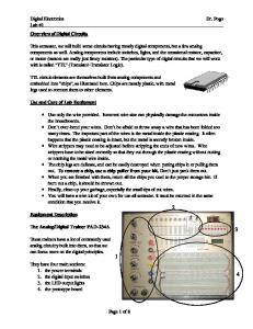
Unit Delay One of the simplest and most important types of delay elements can be modeled
as having the following structure:
Here A is the input signal and B is the associated
output~
The following
statement uses intervals to characterize the desired behavior: In every subinterval of length exactly one unit, the initial value of the
it~- put
A equals the final value of the output B.
The next predicate del formalizes this: A del B
=dec
[!] ((len
41
=
1)
:J
(A--+- B)]
CHAPTER 4--DELAYS AND COMBINATIONAL ELEMENTS Properties: 1=
(A del B)
=
(skip
[A-+ B))*
A
Unit delay can also by viewed as the successive iteration of atomic assignments. This suggests how to implement unit delay by means of looping. F
(A del B)
=
keep(A
=
0 B)
The concept of unit delay can be expressed in semicolon-free linear-time temporal logic. 1=
(A del A)
=
stbA
If a signal is feed back to itself, it is stable. The converse is also true.
§4.2
Transport Delay It is natural to extend the predicate del to cover delays over m-unit intervals:
A delm B
13(/en
=def
=
m
::::>
[A-+ B])
Breuer and Friedman [10] refer to this as transport delay.
Properties: F
(A del 0 B)
=
(A ~ B)
Zero delay is equivalent to temporal equality. 1=
A del 0 A
A signal has zero delay to itself. F
(A delm B
1\
B deln G)
::::>
A delm+n C
Delay is cumulative. I=
{A, B) delm {A', B')
=
(A delm A'
1\
B delm B')
Delay between pairs is equivalent to component-wise delay. This generalizes to lists of arbitrary length. 42
CHAPTER 4--DELAYS AND COMBINATIONAL ELEMENTS
§4.3
Functional Delay Often, one signal receives a delayed function of another. The following ex-
amples illustrate this and are based on the predicate del although the other delay models later presented can also be ·used.
Examples:
Concept
Formula
X keeps on being complemented
(..,X) del X
B either accepts A or itself, depending on X
[if (X= 1} then A else B] del B
N keeps on doubling
2N del N
A receives a delayed f(A, B)
f(A,B) del A
I keeps decrementing by 1
I del (I+ 1)
.
Here is the description of a system that runs the variable I from 0 to n and simultaneously sums I into J:
beg(!= 0
A
J
= 0)
A
[(I+ 1) del I]
A
((J + !) del J]
Properties: t=
[f(A) delm B
A
g(B) deln c] ::) g(f(A)) delm+n c
Functional composition applies. t=
{..,X) delm Y
=
X delm (..,Y)
Bit inversion can occur either on the input or output. I=
[(..,X) delm y
A
("""~Y)
deC"
z]
:J
Two inverters cancel. 43
X dezm+n
z
A
halt(!= n)
CHAPTER 4-DELAYS AND COMBINATIONAL ELEMENTS
§4.4 Delay Based on Shift Register An (m + 1)-bit vector R acting as a shift register can be specified as follows:
R[O] del R(1]
A ••• "
R(m - 1] del R(m]
Over each unit of time, the contents of R shift right by one element. That is, the value of R[O] is passed to R[1] and so forth. This description is more formally expressed by means of quantification:
Vi E [0, m - 1]. (R[i] del R[i + 1]) The next formula has the same meaning but is more concise: · R[O tom - 1] del R[1 tom), where the vector R(O tom- 1] by definition equals {R(O}, ... , R[m- 1]}. The following property shows how to achieve an m-unit delay by means of such a shift register: I=
R[O tom- 1] del R[l tom]
:::>
R[O] delm R[rn]
This suggests an implementation of A delm B of the form A shdel''R B:
A ahdel''R. B
=der
(A~ R(O]'A
R[m) ~ B " R(O tom- 1] del R[l tom])
Here, the value of A is fed into R[O] and B receives the value R[m]. The correctness of this implementation is given by the following property: I=
A shdel"; B :::> A delm B
We can localize R in the formula A shdelR, B by defining a variant A shdelm B that existentially quantifies over R:
A shdelm B
.
def
3R.[(R: signazm+t) 44
1\
(A shdel'R. B)]
CHAPTER 4-DELAYS AND COMBINATIONAL ELEMENTS Here the construct
R: signalm+l constrains R to being a vector of m
+ 1 signals.
This notation will be described in
more detail in the next chapter. Note that R is assumed to exist without necessarily being externally visible to an observer. The quantifier's effect on seeping is similar to that of a begin-block in a conventional block-structured programming language. We call A shdelm B an external specification of the implementation. In fact, this is logically equivalent to the basic delay predicate A delm B as the next property states: I=
A shdelm B
=
A delm B
Basically, the proof that shdel implies del follows from the property (*) given above. The converse requires demonstrating that some R exists. Perhaps the easiest way to do this is by direct construction. At each instant of time, the values of the
m + 1 elements of R can be those of the next m
R(i] ~ 0 m-i B,
+ 1 values of B
in appropriate order:
for 0 ~ i ~ m
The output value R[m] always equals the expression 0
B's current value. Similarly, R[O] always equals
°B, which is defined to be
om B,
that is, the value B will
have m units later. This technique works even if the interval has length less than
m.
§4.5
Variable Transport Delay A batch of delay elements may have varying characteristics although each
individual device is rather fixed in its timing behavior. The predicate A vardelm,n B specifies that A's value is propagated to B by transport delay with some uncertain factor between m and n: A vardelm,n. B
=deC
3i E [m, n]. (A deli B)
45
CHAPTER 4-DELAYS AND COMBINATIONAL ELEMENTS
§4.6
Delay with Sampling Digital circuits often require that inputs remain stable and be sampled for some
minimum amount of time in order to ensure proper device
~peration.
The delay
model A sadel B has this characteristic: A sad elm B
l!1 [( stb A
=def
1\
len ~ m) :::> fin(A
= B)]
Here the input A must be stable at least m units of time for the output B to equal A. Behavior during changes in A is left unspecified. The properties below illustrate
two other ways of expressing sadel. We present them to demonstrate other possible styles: I=
A sadelm B -
I=
A sadelm B _ [tstbm A~ beg( A= B)]
[!](tstbm A :::> fin(A =B))
Properties: A del"" B :::> A sadel"" B
I=
Basic delay implements sampling-time delay. A sadelm B
I=
= (tstb
m
A ~ [beg(A
=
B)
1\
A blk B])
Once the device stabilizes, the input A blocks the output B. The predicate sadel can be extended to associate some factor with the blocking ofBbyA:
A sadelm,n. B
=dcf
( tstbm A~
[beg( A
=
B)
A
A blkn. B])
In a sense, m is the maximum delay and n is the minimum delay.
§4.7 An Equivalent Delay Model with an Internal State A related delay model Astdel';'n B is based on a bit flag X that is set to 1 after the input A has been held stable m units. Whenever X is 1, the input A equals the 46
CHAPTER 4-DELAYS AND COMBINATIONAL ELEMENTS output B and blocks X, which in turn blocks B by the factor n: A stdel';'n B · Gl([stb A A
=def
1\
len ~
lB( beg(X
=
m] ::) fin(X
=
1))
1) ::> [beg(A =B) " A blk X
1\
X blkn B])
In the manner described earlier, we internalize X by existentially quantifying over it:
=
A stdelm,n B
3X. (A stdelr;,n B)
This external form is in fact logically equivalent to A sadelm,n B:
t=
A stdelm,n B
=
A sadelm,n B
The following construction for X can be used: X~
(il [beg(A =B)
" A blkn B] then 1 else 0)
The right hand expression is not a signal but is converted to one as outlined in the next chapter. There are a variety of specifications that use different internal signals such as X and yet are externally equivalent.
§4.8
Delay with Separate Propagation Times for 0 and 1 Sometimes it is important to distinguish between the propagation times for 0
and 1. The following variant of sadel does this by having separate timing values for the two cases. The delay's input and output are both bit signals. X sadel01 m,n Y
A
=def
m] ::) fin(X
r3{[X
~
0
A
len
G([X
~
1
A
len ~ n] ::> fin(X
~
= Y)) =
Y))
Property: I=
X t?adel01 m,n Y
:::> X sadelmax(m,n) Y
The separate propagation times can be reduced to those for the more general form of sampling-time delay by using the larger of the two parameters.
47
CHAPTER 4-DELAYS AND COMBINATIONAL ELEMENTS
§4.9
Smooth Delay Elements It is possible to specify that between times when the delay element is steady, if
the input changes smoothly, then so does the output. We call such a device a smooth delay element. This type of delay has utility in systems that must propagate clock signals without distortion. Here is a predicate based on the earlier specification stdel: A smdel''X'n B
=deC
A stdelx'n B A
~([beg(X
=
1)
A
fin(X
=
1)
A
smA] .:) smB)
The external form quantifies over X:
A smdelm,n B
§4.10
3X. (A
=def
smdel~,n
B)
Delay with Tolerance to Noise
Sometimes it is important to consider the affects of transient noise during signal changes. A signal A is almost smooth with factor l if A is continuously stable all but at most l contiguous units of time: stb A; (len ::s;; l); stb A
The delay model toldel is similar to smdel but has an additional timing coefficient l for showing how almost smooth input changes result in smooth output transitions:
A toldel";.'"'' B
=del
A stdel';'n B 1\
IB [( beg(X = 1)
A
fin( X= 1)
A [ stb
A; (len ~ l); stb A]) :) sm B]
From this we can obtain the external form A toldelm,n,L B
The predicate smdel is a special case of toldel with a noise tolerance of 1 time unit:
t=
A smdelm,n B
=
A toldelm,n,l B 48
CHAPTER 4-DELAYS AND COMBINATIONAL ELEMENTS
§4.11
Gates with Input and Output Delays
One might specify an and-gate with both input and output delays as follows: (X,X')saandm,ny
=def
3Z,·z'.[X sadelmz
A
X' sadelm Z'
1\
(Z
1\
Z')sadel,.Y]
Here a delay exists from the input X to an internal signal Z and another delay exists from X' to Z'. The bit-and of Z and Z' is propagated to Y. The input delays are given by m and the output delay by n. If we choose to ignore input delays, the model reduces to a single occurrence of sadel: t=
(X, X') saandO,n
=
(X
X') sadeln Y
1\
If the internal propagation is modeled by transport delay, things are even
simpler. Here is an and-gate specified in this manner: (X, X') tandm,n. Y
=det
The predicate tand t=
§4.12
simpli~es
{X,X') tandm,n Y
3Z, Z'. (X del"" Z
A
X' delm Z'
A (Z A
Z') de ln. Y]
even if the internal input delay m is not zero:
=
(X
A
X') dezm+n Y
High-Impedance
Digital devices sometimes use the phenomenon of high-impedance as a decentralized means for sharing a common output among several sources. Each source has its own enabling signal which, when on, causes data to pass to the output. When the enable signal is off, the connection "disconnects" or "floats." Pass transistors in MOS semiconductor technology and tri-state drivers in TTL exhibit this kind of
behavior. See Gschwind and McCluskey [17] or Mead and Conway [32] for details. The predicate A pass x B specifies the connection of the signals A and B when the bit signal X is 1:
A passx B
=dec
8((X 49
= 1)
::> (A= B))
CHAPTER 4-DELAYS AND COMBil'TATIONAL ELEMENTS Thus the pair of devices
(A passx B)
1\
(A' pass...,x B)
will pass the signal A to B when X is 1 and will pass the signal A' to B when X is 0. The following formula has the same semantics:
(if [X= 1] then A else A')~ B The predicate pass shows that the key feature of high impedance can be modeled in ITL without the introduction of extra bit values.
Properties: 1=
Apassx B
=· B passx A
A pass transistor is commutative. I=
[Apassx B
A {X~
1)] :::>
(A~
B)
During intervals when the pass transistor is enabled, the input and output are equal. I=
[A passx B
A
B passy C] :::> A pass(x A Y) 0
Pass transitor behavior is transitive.
50
CHAPTER
5
ADDITIONAL NOTATION
This chapter introduces some useful notation that we
nee~
before looking at
more complicated devices.
§5.1
Reverse Subscripting Because some of the devices we present deal with numbers and their repre-
sentation as bit vectors, it is convenient to occasionally adapt an alternative subscripting order. Subscript~ on a vector V = (vo, ... , vn) normally range from 0 on the leH ton on the right. The construct V[i) follows this style. However,. in order to simplify reasoning about the correspondence between a bit vector and its numerical equivalent, a slightly different convention is sometimes used. The alternative notation V{i} indexes V from the right with the right-most element having subscript 0. For example:
{1, 0, 5){0} = 5, f
{1, 0, 5}{1}
f
=
0,
{1, 0, 5){2} = 1 f
For a vector V and i ~ j, the expression V {i to j} forms a new vector out of the elements indexed from i down to
i.
H i < j, the empty vector is returned. For
example,
{0, 9, 4, 2}{3 t.o 1} = {0, 9, 4},
{0, 1}{0 t.o 0} = {1}, 51
{3, 1," 0, 1){1 t.o 2} =
{)
CI-IAPTER 5-ADDITIONAL NOTATION
§5.2
Conversion from Bit Vectors to Integers The function nval converts a bit vector to its unsigned numerical value. For
example, nval( (0, 1, 1}) = 3,
nval((l, 1, 0, 0})
=
12
The following definition of nval can be used: nval(X)
2:
=tter
(2i · X{i})
Osi BasicAdder(G)
where the tuple G has exactly the following fields and connections to A and B:
II B.lnl A.ln2 II B.ln2
C.Inl
~
C.In2
~
C.Ci
~
B.Ci
C. Out
~
A. Out
C.Co
~
A.Co
C.n
-
A.n+B.n
C.lat
-
min(A.lat, B.lat)
C.prd
-
A.prd + B.prd
A.In1
II B. Out
Here A contains the most significant bits and B contains the least significant ones. The operator
II appends two lists together.
58
CHAPTER 6-ADDERS
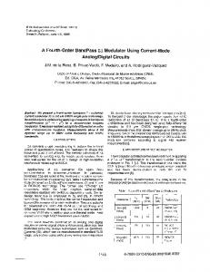
§6.2 Adder with Internal Status Bit An adder of length n can be defined to include an internal status bit in the manner of the delay model stdel. Here is the device structure:
Inl: Bit"=} ln2:Bit"=}
=}Out: Bit" Status: Bit -..Co: Bit
Ci: Bit-+
n, prd, lat
The specification given below is externally equivalent to BasicAdder.
Definition of StatusAdder:
StatusAdder(A)
=def
StatusAdderStructure(A) A [!)
A
Add(A)
l!l Steady(A)
Definition of StatusAdderStructure:
StatusAdderStructure(A)
=det
A: struct[ (Inl, In2): Bitn, Ci: Bit
%Inputs
Out: Bitn, Co: Bit
%Outputs
Status: Bit
%Internal
n: nat, ( lat, prd): time
%Parameters
] 59
CHAPTER 6-ADDERS Definition of Add:
After the inputs remain stable long enough, their sum is propagated to the outputs and the status bit equals 1. Add(A)
=der
( s.tb{lnl, ln2, Oi)
A
len ~ prd)
:::) fin([Status
= 1]
1\ ( nval({ Co)
II
Out)= nval(Inl) + nval(In2)
+ Ci])
Definition of Steady:
Whenever the signal Status is 1, there is a certain amount of blocking from the inputs to it and the outputs. Steady(A)
=def
beg( Status = 1) :::) · [(In1,In2, Ci} blk Status
§6.3
A
{Inl,In2, Ci) blklo.t (Out, Co)]
Adder with More Detailed Timing Information Further timing details can be accomodated as we now demonstrate. Suppose
each input has its own propagation time. This can be specified as follows:
Definition of DetailedAdder:
DetailedAdder(A)
=det
DetailedAdderStructu.re(A) " l:!l Add(A)
60
CI-IAPTER 6-ADDERS
Definition of DetailedAdderStructu.re .·
In this adder, there is a separate parameter for each input's propagation time. DetailedAdderStructure(A)
=def
A: struct[ (Inl, In2): Bit"', Ci: Bit
%Inputs
Out: Bit"', Co: Bit
%Outputs
n: nat,
%Parameters
prd: (Inl, In2, Ci): time,
lat: time
] We use the construct prd: (Inl, In2, Ci): time ·
to indicate that prd has three subfields accessible as prd.Inl, prd.In2 and prd. Ci.
Definition of Add: IIere each input has its own time for stabilizing.
Add(A)
=det
( tstbprd.Inl
Inl
A
tstbprd.In 2 ln2 A tstbprd.Oi
~[nval((Co} II Out)= (nval(Inl) A ( Inl,
The sampling requirements
~an
Ci)
+ nval(In2) +
In2, Ci} blklat ( Co, Out)]
also be given in a less redundant form:
Vfield E '{Inl, In2, Ci}.
(tstbprd(field]
Recall that '{1n1, In2, Ci} represents the set
{' Inl,' In2,' Ci}.
61
A[field])
Ci)
CHAPTER 6-ADDERS
§6.4 Adder with Carry Look-Ahead Outputs Long adders usually have extra control signals to speed up the propagation of carry bits. One technique is called carry look-ahead (see [17]) and produces sum and carry outputs as well as two bit signals Gen and Prop. The structure is as follows:
Out: Bit'"
In1: Bit'"'=}
Co: Bit
In2: Bitn=}
Ci: Bit
Prop: Bit
n, prd, lat The bit signal Gen is 1 iff the result of adding In1 and In2 will generate 1 as carry no matter what the carry input Ci is. The bit signal Prop is 1 iff the carry input Ci
will be propagated unchanged to the carry output Co. Because both Gen and Prop can be computed without the carry input, they need not wait for carry rippling. Definition of CarryLookAheadAdder:
CarryLookAheadAdder(A)
=def
CLAAdder Structure (A)·· A [!I
Add(A, output),
for output E '{Out, Co, Gen, Prop}
The last line is equivalent to 8 Add(A,' Out) " G Add(A, ' Co) "
[!]
62
Add(A, ' Gen) "
[!]
Add(A, 'Prop)
CHAPTER 6-ADDERS Definition of CLAAdderStructure:
CLAAdderStructure(A)
=det
A: struct[ {Inl, In2): Bit n, Ci: Bit
%Inputs
Out: Bitn, (Co, Gen, Prop): Bit
%Outputs
n: nat,
%Parameters
prd: (Out, Co, Gen, Prop): time, lat: (Out, Co, Gen, Prop): time
The specification gives various propagation and latency times by making prd and lat each have a subfield for every output.
The function inputs shows the inputs used by each output: inputs(A, output) {Ci, In1, In2} {Ci, In1, In2} {In1, In2) {Inl, In2)
outp'Ut
Out Co Gen Prop
As noted earlier, the generate and propagate signals can be computed without reference to the carry input. Definition of Add:
For any selected output, after the appropriate input fields remain stable long enough, the device satisfies the predicate result and the output depends on its associated inputs. Add(A, output)
=def
( stb inputs( A, output)
1\
len ~ prd( output])
~ [result( A, output)
where i
=
1\
inputs(A, output) blki A[ output]]
lat[ output] and the predicate result has the following definition:
63
CHAPTER 6-ADDERS output
result(A, output)
nval( Out)= (nval(Inl) + nval(In2) + Ci) mod 2n Co= carry(n, nval(Inl), nval(In2), Ci)
Out Co Gen Prop
Gen Prop
= =
carrygen(n, nval(Inl ), nval(In2)) carryprop(n, nval(Inl ), nval(In2))
The functions carry, carrygen and carryprop compute appropriate values: carry(n, j, k, ci)
+k+
(j
=def
ci) -7- 2n
carrygen(n,j, k)
=def
if (Vci E {0, 1}.
carry(n,j, k, ci)
=
1) then 1 else 0
carryprop(n,j, k)
=def
if (Vci E {0,1}.
carry(n,i, k, ci)
=
ci) then 1 else 0
Both carrygen and carryprop can be simplified: carrygen(n, i, k) carryprop(n, j, k) =
= if (i + k if (j + k
~
=
2n) then 1 else 0
2n- 1) then 1 else 0
Thus, a carry is generated exactly when the sum of the two numbers
i and k exceeds
the capacity of n bits. Similarly, the incoming carry is propagated if the sum of j and k is the "borderline" value 2n- 1. In practice, a carry look-ahead adder may output Gen and Prop in complemented form as the signals Gen and Prop. If we ignore propagation delay, the adder has the following behavior: Voutput E '{Out, Co, Gen,Prop}.
64
[rn result(A, output)]
CHAPTER 7
LATCHES
A latch is a simple memory element for storing and maintaining a single bit of data. The two inputs Sand R determine what value is stored with S standing for
Set and R standing for Reset. When the latch is steady, the outputs Q and Q are complements. Note that the bar in "Q" is part of the name and not an operator. Such elements are among the simplest storage devices· that can be constructed out of TTL gates and provide a basis for building counters and other sequential components.
§7.1
Simple Latch Here is one possible latch specification:
(S,R) latchm,n (Q, Q) [3 ( ( S
~0
A
R ~1
~( beg[Q 1\
[!] ( ( S
::=:::::;
1
1\
=def
=
0
R ~0
~( beg[Q
=
len ~ m)
1\
1
1\ A 1\
(J
=
1]
1\
S blkn {Q, Q})]
1\
R blkn (Q, Q))]
len ~ m)
Q = 0]
For example, the specification states that after S is 1 and R is 0 for at least m units of time,
Q equals 1, Q equals 0 and R blocks both with factor n. That
is, the outputs are stable as long as R remains "inactive" at 0, independent of S's behavior.
65
CHAPTER 7-LATCI-IES Such a latch can be constructed out of two nor-gates that feed back to one another: t=
[-,(R v Q) sadelm,n Q
1\
_,(S v Q) sadelm,n Q
1\
n ~
1]
:) _[(S,R) latch 2 m,n (Q, Q)] For example, to set Q to 1 and Q to 0, ·we keep R at 0 and S at 1. After m units of time, Q equals 0 and after 2m units of time, Q equals 1. At this point both Q and
Q are stable as long as R remains equal to 0. The gates' blocking factor n must be nonzero in order to achieve a feedback loop that maintains the values of Q and Q.
§7 .2
Conventional SR-Latch The latch specification now given has separate parts for entering and main-
taining a value in the device. The following sort of table is often given to describe operation for various input values:
s 1
0 0 1
Q 1 0 1 0 unchanged unspecified
Q
R 0 1 0 1
.,
For example, assuming unit delay, the behavior of Q can be expressed by the formula
13( skip
::>
([beg(S
=
_,R) ::> (S--.. Q)) " [beg(S
=0"
R
= 0)
The following predicate SRLatch goes into more details on timing.
Definition of SRLatchStructure: The latch includes the internal bit flag Status:
SRLatchStructure(L)
=def
L: struct[
(S, R): Bit
%Inputs
(Q, Q): Bit
%Outputs
Status: Bit
%Internal
(prd, lat): time
%Parameters
] 66
:::>
stb Q])]
CI-IAPTER 7-LATCHES
We use Status to indicate when the device is steady.
Definition of SRLatch: The latch can be set to 1, cleared to 0, disabled or kept steady.
SRLatch(L)
=der
SRLatchStructure(L) A
G Store(L, i),
A
G Disable(L)
A El
fori E {0, 1}
Steady(L)
· The formula . f!l Store(L, i),
for i E {0, 1}
is equivalent to
13 Store(L, 0) " Gl Store(L, 1)
Definition of Store: This definition uses the static variable i to determine the value to be stored:
Store(L, i)
=def
[(S ~ i)
A
(R
R::1
--.i)
A
:> fin[(Status =
(len ~ prd)]
1)
A
(Q = i)]
Alternatively we can omit i by using a formula such as
[stb(S,R}
A
beg(S
=
--.R)
A
(len~ prd)]
:J
fin[(Status
=
1) " (Q
=
S)]
This works because S and R must be complements when setting or resetting and S matches the value stored in Q.
Definition of Disable: If the device is initially steady and the two inputs S and R smoothly become 0 for a period of sufficient length, the device remains steady and the outputs are 67
CHAPTER 7-LATCI-IES stable.
Disable(L)
=def
(beg(Status :::>
=
1)
A
smo,prd(S,R)
[fin(Status
=
1)
1\
A
fin(S
=
0
1\
R
=
0)]
stb(Q, Q)]
Definition of Steady: When the flag Status equals 1, the outputs Q and Q are complements. In addition, the flag and outputs depend on the two inputs S and R.
Steady(L)
=def
beg( Status = 1) :::> (beg((J
=
-.Q)
1\
(S,R) blk Status
I\
(S,R) blklat (Q, Q)]
Constructing an SR-latch The next property shows how the first latch described implements a conventional SR-latch: t=
[(S,R) latchm,n (Q, Q)]
:::>
SRLatch(L)
·where the tuple L has exactly the following fields and connections:
s
L.S
~
L.R
~
R
L.Q
~
Q
L.Q
~
Q
L.prd
-
m
L.lat
-
n
and L.Status is constructed as follows: L.Status ~
if (3i E {0, 1}. [Q
=
i
1\
Q = ..,i
1\
(S, R}[i]
=
0
1\
((8, R)[i]) blkn (Q, Q)]) then 1 else 0
At all times, L.Status is set to 1 if Q and Q have complementary values and are blocked by S if Q
=
0 and by R if Q
=
1. The quantified variable i is used to
determine the values of Q and Q.
68
CHAPTER 7-LATCI-IES
§7 .3
Smooth SR-Latch The predicate Store in the specification SRLatch can be modified to include
additional details regarding smooth transitions. As before,
8to~e
shows how to enter
0 or 1 into the latch. In addition, if the status bit is initially 1 and the inputs S and
R are smooth, the outputs are also smooth. Notice that there is no requirement that Q and
Q change at exactly the same time. Store(L, i)
=def
[tstbprd(S, R) :::>
fin[(S
1\
[fin( Status 1\
§7.4
=
= i) 1
1\
1\
Q
([sm(S, R)
(R
= A
= -.i)}]
i) beg( Status
=
~)] :::>
sm(Q, Q))]
D-Latch A simple D-latch has one inp11t pin to selectively enable the latch to accept data
and another to indicate the actual value to be stored. The operation corresponds roughly to the following
t~ble,
where E and Dare the enable and data inputs, and
Q and Q are the outputs:
E
D
1
0
1
1
0
Q 0
1 1 0 unchanged
When E is held active at 1, D's value is propagated through the device as through a delay element. When E is 0, the device maintains whatever value is stored, independent of D. The formula below uses unit-delay to describe this:
(if [E
= 1] then (D, -.D)
else (Q, Q)) del (Q, Q)
If we just look at the behavior of Q, this reduces to
(if [E
= 1] then D
else Q) del Q
The D-latch is also referred to as a transparent latch because when E is enabled, the input data passes through to the output. 69
CIL-\PTER 7-LATCHES
Definition of DLatch: As with the SR-latch, the specification has predicates for examining, modifying and disabling the device:
DLatch(L)
=def
DLatchStructure(L} 1\
G Store(L)
1\
G Disable(L)
1\
G Steady(L)
DLatchStructure(L)
=def
L: struct[
(E, D): Bit
%Inputs
(Q, Q): Bit
%Outputs
Status: Bit
%Internal
(prd, lat): time
%Parameters
Definition of Store: When the latch is enabled, the data signal D's value propagates to the output
Q. Store(L)
=deC
[(E ~ 1)
A
stb D
A
{len ~ prd)]
:J
fin[(Status
= 1)
1\
(Q =D)]
Definition of Disable: If the enable signal drops to 0 and the data remains stable, the latch becomes disabled and retains the value it was set to.
Disable(L) - [tO,prdE
=der A
:J
stbD
A
beg(Status = 1)]
[fin(Status
=
1) 70
A
stb{Q, Q)]
CHAPTER 7-LATCHES Definition of Steady: Whenever the signal Status equals 1, the outputs Q and Q are complements of each other. If E is di~abled, it blocks the status flag and outputs. When E is enabled, the flag and outputs are blocked by E and the incoming data signal D.
Steady(L)
=dcf
beg(Status
= 1)
:::) [beg( Q = •Q)
1\
V blk Status
A
V blklat (Q, Q)]
where V is a function of the enable signal's initial value:
E 0
V (E)
1
(E,D)
Building aD-latch AD-latch can be implemented by connecting a suitable combinational interface to the inputs of an SR-latch. The interface has inputs E and D and outputs Sand
R with stable-state behavior given by the following table:
E
D
8
R
1
0 1
0
1
1
0
0
0
1
0
When the interface is enabled with E at 1, the data signal D controls S and R for clearing or setting. If E is 0, both S and R are deactivated. The interface has the following description: Definition of DLinterface:
DLinterface(A)
=det
DLinterfaceStructure(A) A [!)
Store(A)
A [!]
Disable(A)
A [!)
Steady(A)
71
CHAPTER 7-LA.TCI-IES Definition of DLinterfaceStructure:
DLinterfaceStructure(A)
A: struct[ (E, D): Bit
%Inputs
(S, R): Bit
%Outputs
Status: Bit
%Internal
(prd, lat): time
%Parameters
] Definition of Store:
When the device is enabled, the outputs eventually reflect D and its complement. This is done so that any connected SR-latch will be actively set to D's value. Store(A)
=def
[E ~ 1
stb D
1\
:J
1\
(len ~ prd)]
·fin[( Status = 1)
(S =D)
1\
1\
(R =..,D)]
Definition of Disable:
When the interface is disabled, both outputs smoothly change to 0 so that any connected SR-latch retains its value. Disable(A)
[! O,prd E
=def 1\
:J
stb D
1\
beg( Status
[fin( Status
=
1
1\
S
= 1)]
=
0
1\
R
= 0)
1\
sm(S, R}]
Definition of Steady:
When the device is steady, the status bit and outputs are blocked by the appropriate inputs: Steady(A)
=def
beg(Status
=
1)
:J
(V blk Status
72
1\
V blklat (S,R})
CHAPTER 7-LATCI-IES where V is based on the initial value of E:
E
V
0 1
(E) {E,D)
Combining the interface with SR-latch The following predicate shows how to connect the interface's outputs to the inputs of an SR-latch:
DLatchlmplementation(A, L) DLinterface(A)
A
=deC
SRLatch(L)
" (A.S ~ L.S) " (A.R ~ L.R) The next property states that this implementation results in a D-latch: ~ . DLatchlmplem~ntation(A, L) ::> DLatch(M)
where M.E
~
A.E
M.D
~
A.D
~
L.Q
M.Q M.Q
~
L.Q
M.Status
~
A.Status
M.lat
-
A.lat
M.prd
-
A.prd + L.prd
A
L.Status
+ L.lat
The interface itself can be built from combinational gates based on the steadystate formula
We omit the details.
73
CILA.PTER 7-LA.TCHES Introducing a hold time In practice, a D-latch's data input need not be held stable during the entire period when the D-latch is disabled and the enable signal drops. This can be formalized by adding a hold-time parameter hld and redefining D£sable to incorporate it:
Disable(L) [tO,prdE
=clef 1\
::J
E blkhld D
[fin(Status
1\
beg(Status = 1)]
= 1)
74
1\
stb(Q, Q)]
CHAPTER
8
FLIP-FLOPS
§8.1
Simple D-Flip-Flop The simple D-ftip-flop described here has as inputs a clock and a data signal.
The overall structure is given by the following diagram:
Q: Bit
Ck: Bit
---+ Q:
D:Bit
Bit
( cl, c2, c3, hid, lat): time
H we ignore the clock input Ck and assume unit delay, the flip-flop behavior
can be described by the formula
(D del Q] " ((..,D) del Q] The predicate SimpleDFlipFlop given below takes a more detailed look at clocking and propagation. 75
CIIAPTER 8-FLIP-FLOPS Definition of SimpleDFlipFlop:
SimpleDFlipFlop(F)
=der
SimpleDFFStructure( F) 1\
Defin~'tion
G Store(F, i),
for i E {0, 1}
of SimpleDFFStructure:
SimpleDFFStructure(F)
=clef
F: struct[ ( Ck, D): Bit
%Inputs
(Q, Q): Bit
%Outputs
( cl, c2, c3, hld, lat): time
%Parameters
Definition of Store:
The predicate Store shows how to store a value in the flip-Hop: Store(F, i)
=clef
(t! cl,c 2 ,c 3 Ck
A
Ck blkhld D
~[beg(Q = i
1\
1\
beg(D
Q = ..,i)
A
=
i)]
Ck blkla.t (Q, Q}]
The Hip-Hop specificati9n can be generalized into a multi-bit register by representing the input data and the output as vectors of the appropriate length. If still more detail is desired, such a register can be viewed as a collection of one-bit Hip-flops, each with its own status bit. Incidentally, it is easy to connect, say, the output of one device to the clock input of another. Here is an SimpleFlipFlop(F)
A
SimpleFlipFlop( G)
76
1\
ex~ple:
(F. Q ~ G. Ck)
CHAPTER 8-FLIP-FLOPS
§8.2
A Flip-Flop with More Timing Information The predicate DFlipFlop presented below includes additional timing details.
When the clock signal rises, the current value of the data line is stored in the device. Falling clock edges leave the stored value unchanged. This description also takes a more precise look at the process of setting up the input data prior to triggering. When the internal flag Status equals 1, as long as the clock is stable, the output bit
Q remains stable and is also available in complemented form as Q. Definition of DFlipFlop:
Here is the main predicate: DFlipFlop(F)
=det
DFlipFlopStructure( F) 1\
13 Store(F)
1\
13 Nontrig(F)
1\ [!)
Steady(F)
Definition of DFlipFlopStructure:
DFlipFlopStructure(F)
=det
F: struct[ ( Ck, D): Bit
%Inputs
(Q, Q): Bit
%Outputs
Status: Bit
%Internal
(stp, prd, hld, lat): time
%Parameters
Definition of Store:
The predicate Store shows how the clock triggers the flip- flop to accept a new value. The data must not change until after the clock goes high. Before the actual
77
CHAPTER 8-FLIP-FLOPS triggering, the clock and data are set up by being initially stable for at least stp units of time. The actual clocking is given by the predicate Trigger.
Store(F)
=clef
( stb( Ck, D)
1\
[len 2:: stp 1)
.....:.?>
Trigger( F)
If desired, we can have separate set-up times for the clock and data inputs. For example, the value stp. Ck can give the time required to set up the clock. The following formula demonstrates one way to do this:
( tstbstp.G k Ck
1\
tstbstp.D D) ~ Trigger( F)
Incidentally, an externally equivalent D-flip-flop specification can be given that includes an additional internal field SetupStatus equaling 1 whenever the inputs have been set up.
Definition of Trigger: Mter the clock rises and triggers the device, the data input D must remain stable for at least the hold time specified by the parameter hld. If this condition is fulfilled, the device ends up steady with Status equaling 1 and Q receiving D's initial value.
Trigger(F)
=clef
(iO,prdCk
A
Ck blkhld D) ::> [fin(Status
=
1)
A
(D-+ Q)]
Definition of Non trig: If the clock has a falling or non-triggering edge and the device is initially steady then the device remains steady and outputs are stable.
Nontrig(F)
=clef
[! O,prd Ck
1\
= 1)] = 1) A
beg( Status
::> [fin(Status
78
stb(Q, Q}]
CHAPTER 8-FLIP-FLOPS Definition of Steady: Whenever the status bit equals 1, it and the outputs remain stable as long as the clock does, independent of the behavior of the data input. The outputs are complements.
Steady(F)
=dcf
beg( Status
=
1)
:::> [beg( Q =
-.Q)
1\
Ck blk Status
1\
Ck blklat {Q, Q)]
If desired, the latency factor can be a function of the initial value of the clock or even the currently stored value. Comparison of the predicates SimpleDFlipFlop and DFlipFlop
The next property shows how to reduce the predicate DFlipFlop to the predicate SimpleDFlipFlop presented earlier: F
DFlipFlop(F) ::> SimpleDFlipflop( G)
where G is constructed from F as follows:
G[field]
~
F[field],
G.cl
-
F.stp
G.c2
-
F.prd
G.c3
-
F.prd
G.hld
-
F.hld·
G.lat Simplifying the
-
for field E '{ Ck, D, Q, Q}
F.lat
predicat~
Store in DFlipFlop
By merging the processes for setting up and triggering the flip-flop, we can eliminate the predicate Trigger and define Store as follows:
(i'stp,prdCk
1\
Ck blkhld D) :::> [fin(Status
=
1)
A
(D--:-+- Q)]
Here the clock input is set up at least stp units of time. Because the clock blocks the data input D, D is also set up. 79
CHAPTER 8-FLIP-FLOPS
§8.3 Implementation of D-Flip-Flip AD-flip-flop can be constructed out of two components in a manner similar to building aD-latch. The first component, known as the master latch, serves as an interface between the clock and data inputs on one hand and the second component, the slave latch, on the other. The slave provides the flip-flop's outputs. There are four key time periods in the overall Hip-flop operation: clock is 0, clock rises from 0 to 1, clock is 1, and clock drops from 1 to 0: • When the clock is 0, the master latch disables the slave, which maintains whatever value was previously stored. At this time, the clock and data inputs can be set up for clocking in a new bit. • Upon the clock transition from 0 to 1, the master latch itself stores the incoming data signal and actively propagates it to the slave. The slave in turn adjusts the outputs to reflect the new data. • As long as the clock remains at 1, the master continues to transmit the stored
value to the slave. •. When the clock drops from 1 to 0, the master disables the slave, leaving the stored value undisturbed. At this point, the cycle of clocking can be repeated.
Specification of the master latch The master latch has the following structure:
Ck: Bit-+
-+8:
Bit
D: Bit-+
-+R:
Bit
( stp, hld, prd, lat): time
80
ClfAPTER 8-FLIP-FLOPS The timing parameters have the same form as in the flip-flop description since the master device has the clock and data signals as inputs.
Master(M)
=def
MasterStructure( IV!) 1\.
r!l Store(M)
1\ [!)
Non trig( M)
1\ [!]
Steady( M)
Definition of MasterStructure:
Master Structure( M)
=def
M: struct[ ( Ck, D): Bit
%Inputs
(S, R): Bit Status: Bit
%Outputs %Internal
( stp, hld, prd, lat): time
%Parameters
] Definition of Store: The data value present when the clock rises determines the S and R outputs.
Store( M)
=clef
(stb{Gk,D}
1\
len 2::
stp)~
Trigger(M)
where the predicate Trigger is defined as follows:
Trigger( M)
=def
{ to,prd Ck A
Ck blkhLd D)
::) [fin( Status
=
1) 81
A
(D ~ S)
A ( .,D
--.. R)]
CHAPTER 8-FLIP-FLOPS
Definition of Non trig: If the master latch is initially steady, then after the clock drops, both S and
R become smoothly disabled at 0.
Nontrig( M)
=clef
[.1. O,prd Ck
beg( Status= 1)]
A
:::> [fin([S
= 0]
[R
1\
=
0]
A
[Status= 1])
A
sm{S, R}]
Definition of Steady:
When the master latch is steady, the status flag and the outputs are blocked by the clock. Steady( M)
=clef
beg(Status
=
1) :::> [Ck blk Status
A
Gk blklat {S,R}]
Combining the latches The next predicate shows how the master and slave latches are combined to implement a D-Hip-fiop. We use an SR-latch as the slave. DFFimplementation(M, L) Master(M)
A
=det
SRLatch(L)
" (M.S ~ L.S) " (M.R ~ L.R) The mapping from the latches to the flip-flop takes the following form: t=
DFFimplementation(M, L) :::> DFlipFlop(F)
where the tuple F is constructed as follows: F.Ck
~
M.Ck
F.D
~
M.D 82
CHAPTER 8-FLIP-FLOPS
F.S
::::::::s
L.S
F.R
~
L.R
F. Status
~
(M.Status
F.stp
-
M.stp
F.prd
-
L.prd + M.prd
F.hld
-
M.hld
F.lat
§8.4
A
L.Status)
L.lat + M.lat
D-Flip-Flops with Asynchronous Initialization Signals Integrated circuits such· as the TTL 7474 chip [48] contain D-fiip-fiops with
extra ·inputs for initialization. Since these pins are used more or less independently · of the clock, they are called asynchronous. The device considered here has a single asynchronous input Clr:
Ck: Bit
Q:Bit Status: Bit
D:Bit
-+-Q: Bit
Clr: Bit
stp, prd, hld, lat
Definition of AsynchDFlipFlop:
The specification has predicates for operating the clock and clear signals:
AsynchDFlipFlop(F)
=dec
AsynchDFFStructure(F) 1\ [!]
Use Clock( F)
1\
13 UseClear(F)
A
13 Steady(F)
83
CHAPTER 8-FLIP-FLOPS
Definition of Aa7JnchDFFStructure:
Aa11nc hDFFStructure( F)
=det
F: atruct[ ( Ck, D, Clr): Bit
%Inputs
(Q, Q): Bit
%Outputs
Status: Bit
%Internal
( stp, prd, hld, lat): time
%Parameters
] Definition of Use Clock:
During periods when the input Clr equals 0, the device acts according to the earlier specification DFlipFlop: Use Clock(F)
=det
( Clr ~ 0) ::> DFlipFlop(G)
where G contains exactly the following fields ofF: Ck, D, Q, Q, Status, stp, prd, hld, lat Definition of Use Clear:
When the clock is stable, the input Clr can be used to initialize the fiip-ftop: UseClear(F)
=del
stb Ck ::> [Clear( F)
A
Disable(F)]
Definition of Clear:
If the input Clr equals 1 long enough, the output Q is zeroed and the device becomes steady: Clear(F)
=del
( Clr ~ 1 " len 2: prd) ::> fin[(Status = 1) /' (Q = 0)] 84
CHAPTER 8-FLIP-FLOPS.
Definition of Di1able: When the device is steady and the input Clr drops to 0, the device remains steady:
Disable( F)
=dat
(~ o,,,.d Clr A beg( Status = 1)] :::> fin [(Status = 1) A stb{ Q, 11}]
Definition of Steady:
When the Hip-flop is steady, the inputs Ck and Clr
togeth~r
block the signals
Status, Q and Q: Steady(F)
=def
beg( Status= 1) :::> [beg(Q
=
85
..,Q)
A (
Ck, Clr) blk (Status, Q, "Q)]
CHAPTER
9
MORE DIGITAL DEVICES
We now consider techniques for describing and reasoning
~bout
multiplexers,
random-access memories, counters and shift registers.
§9.1
Multiplexer A multiplexer has a number of addressible inputs and can selectively output
any one of them. The device considered below can be optionally disabled, in which •
case it outputs a zero. The general structure is as follows:
Addr: Bit"
In[O): Bit =>Out: Bit
In[2" -1]: Bit E: Bit n: nat,
(prd, lat): time
The device operates roughly according the table below: operation select disable
E 1 0 86
Out
In(loc] 0
CHAPTER 9-MORE DIGITAL DEVICES where loc
=
nval(Addr). If we ignore propagation delay, the multiplexer behaves
according to the formula Out~ (if
[E = 1] then In(nval(Addr)] else 0)
During periods when the device is enabled withE= 1, the formula reduces to Ov.t ~ In[nval(Addr))
Definition of Multiplexer:
The multiplexer's main predicate is as follows: Multiplexer(X)
=der
MultiplexerStructv. re (X) A
IB Select( X, loc ),
1\
1B Disable(X)
for loc E [0, n- 1)
Definition of Multiplexer Structure:
The device has an n- bit vector Addr for selecting one of 2n possible incoming bits of the vector In. MultiplexerStructure(X)
=der
X: struct[ Addr: Bitn, In: Bit< 2 ">,E: Bit
%Inputs
Out: Bit
%Outputs
n: nrd, (prd, lat): time
%Parameters
Definition of Select:
If the enable signal E is held at 1 and the address line and its associated input are stable, the output ends up equal to the input line indicated by the static variable
87
CHAPTER 9-MORE DIGITAL DEVICES
loc. Select(X, loc)-
=def
([E ::=::::s 1]
stb In[loc]
A
1\
[nval(Addr)
~[beg( Out= In[loc])
1\
::=::::s
loc]
A
len ~ prd)
(E, Addr, In[loc]} blklat Out]
Definition of Disable:
Holding the signal Eat 0 clears the output.
Disable(X) (E
::=::::s
0
=der 1\
len ;;::: prd) ~ [beg( Out= 0)
1\
E blklat Out]
Alternative specifications Like the adder discussed earlier, the predicate Multiplexer can be equivalently specified with an internal status bit and predicate Steady. The timing parameters could be made more detailed so that, for example, the
•
parameter select. prd would give the propagation time when using the predicate
Select.
§9.2
Memory The memory described here has the following form
Addr: Bit"'
Data: Bit-+-
Status[O]: Bit
Out(O): Bit
E:-Bit~
n:
nat,
(prd, stp, lat): time There is a series of cells, each associated with status and output bits. At any time, at most one cell can be selected and modified. During this period the remaining
88
CHAPTER· 9-MORE DIGITAL DEVICES cells are left untouched. 'When the enable signal is inactive at 0, no cell can be altered.
If we assume unit delay, the memory behaves as follows:
[if (E = 1) then
alter( Out, nval(Addr), Data). else Out] del Out
where the function alter( Out, i, a) equals a vector whose i-th element equals a and whose remaining elements equal those in Out. The behavior can also be expressed using iteration and an in-place variant of alter: (skip
A
(if (E
=
1} then Alter( Out, nval(Addr ), D) else ( stb Out)])*
where Alter( Out, i, a) sets the i-th element of Out to a and leaves the others unchanged: Alter( Out, i, a)
(alter( Out, i, a) ~ Out]
=def
In practice, a memory has a multiplexer connected to the outputs so that at any time at most a single cell can be read. This technique permits one cell to be written while another is being retrieved. We do not include such multiplexers here. Definition of Memory:
Memory(M)
=der
Memory Structure( M) 1\
Vloc E [0, 2n- 1]. [!]
Enable(M, loc)
1\
1!1 Write(M, loc)
A
I!J Disable(M, loc, mode),
A [!)
for mode E '{selected, not_selec~ed}
Steady( M, loc, mode), for mode E '{disabled, selected, not_selected}
89
CHAPTER 9-MORE DIGITAL DEVICES Definition of Memory Structure:
Memory Structure( M)
=der
M: atruct[ Addr: Bit n., Data: Bit, E: Bit
%Inputs
Out:
%Outputs
Bit( 2 n)
Bit< 2 n)
Status:
%Internal
n: nat, (prd, stp, lat): time
%Parameters
] Definition of Enable: When the memory becomes enabled withE rising from 0 to 1 and a cell does not have the address selected by Addr, the cell's output remains stable.
·Enable( M, loc) •
(f·lfp,prdE
=del A
stbAddr
A
beg[nval(Addr)=tfloc
::> fin[(Status[loc]
=
1)
A
A
Status[loc]=l])
stb Out[loc]]
Definition of Write: "When the device is enabled, the cell addressed by Addr can be written with the value of the data input. .
Write(M, loc)
=def
(len ~ prd " [E ~ 1]
A
s·tb Data " nval(Addr) ~ loc) .
:::> fin[(Statua[loc]
= 1)
A ( Out[loc]
=Data)]
Definition of Disable: Disabling the memory does not affect a steady cell's output. If the cell is currently addressed, both Addr and Data must remain stable until alter E drops. 90
CHAPTER 9-MORE DIGITAL DEVICES Otherwise only Addr need hold. The predicate check, defined below, ensures that the particular location is in the indicated mode.
Disable(M, loc, mode)
(!O,prdE
A
::>
stb U
=def
beg(check(M, loc, mode)
A
[fin(Status[loc] = 1)
where U is as follows:
A
A
(Status(loc]
=
1)])
stb Out[locl]
u
mode selected noLselected
(Addr, Data) {Addr}
Definition of Steady: Steady( M, loc, mode)
=def
beg[(Status[loc] = 1) ::>
A
check(M, loc, mode)]
(V blk Status[loc]
1\
V blkla.t Qu.t[loc])
where the table below gives V as a function of the indicated mode:
v
mode disabled selected not_selected
{E) {E, Addr, Data} {E, Addr}
If a cell is steady, its output is blocked by the signal E and other appropriate inputs
based on whether the device is enabled and whether the cell is the one selected. If the entire memory is disabled, only E blocks the cells. If the memotj is enabled. and the particular cell is the one selected, the cell's output is blocked by the inputs E,
Addr and Data. If however the cell is currently not selected, it is blocked only byE and Addr. This is summarized in the table shown after the definition of Steady. The predicate check, defined below, makes certain that the particular memory location is indeed in the chosen mode of operation.
Definition of check: The predicate check verifies that the given location is in the specified mode of operation:
91
.,
CHAPTER 9-MORE DIGITAL DEVICES mode disabled selected not_selected
§9.3
check(M, loc, mode)
= 1) (E = 1) (E
E=O
1\ 1\
[nval(Addr) = loc) [nval(Addr) ~ loc]
Counters We can model a simple counter by means of addition and unit-delay:
(I+ 1) del I The next formula shows a way to handle initialization:
[if (Clr = 1) then 0 else (I+ 1)] del I If it is only necessary
th~t
the counter is initially equal to 0, the formula below
suffices:
beg(!
= 0)
A
[(I+ 1) del I]
The following example takes finite precision into account:
[(I+ 1) mod 2"] del I Clocked counter
A clocked counter stores a number that can by incremented by 1 modulo some base when the device is triggered. Here is the physical structure: Ok: Bit
Clr: Bit
Status: Bit
Out: Bitn
n, cl, c2, c3 The bina.ry counter considered here has ann-bit output vector and cycles through the numbers 0 to 2n -1. Not all counters are binary. For example, a decade counter has a 4-bit output and cycles through the numbers 0 to 9. The values 10 to 15 are never computed. 92
CI-IAPTER 9-MORE DIGITAL DEVICES Definition of Counter: The predicates Clea·r and In~rement specify how to clear and increment the counter's output.
Counter( C)
=def
CounterStructure( C) A
l!l Clear( C)
A
l!l Increment( C)
A
l!l Steady( C)
Definition of Counter Structure: The device's structure is given below. The internal bit signal Status indicates when the device is in a steady state.
CounterStructure( C)
=det
C: struct[
( Gk, Glr ): Bit
%Inputs
Out: Bit'"
%Outputs
Status: Bit
%Internal
n: nat, ( cl, c2, c3): time
%Parameters
] Definition of Clear: When the clock has a positive pulse and the input Clr equals 1, the device is cleared and ends up steady with Status equaling 1:
Clear(C)
=det
[f l cl,c 2 ,c 3 Ck
A
beg( Clr
=
1)
A
Ck blk Clr]
::) fin[nval( Out)= 0
93
A
Status
= 1)
CHAPTER 9-MORE DIGITAL DEVICES Definition of Increment: If the device is initially steady and the clock is pulsed and Clr equals 0, then
the output vector's numerical value is incremented by 1 modulo 2n. · The device ends up steady. Increment( C)
=def
(t l cl,c 2 ,c 3 Ck
beg( Status
A
=
1
=
Clr
A
::') ([ nval( Out)+ 1] mod 2n
-+
0)
A
Ck blk Clr]
nval( Out)
A
fin{Status = 1])
Definition of Steady: When the bit signal Status equals 1, the clock input blocks both Status and Out. The blocking factor lat is associated with Out. Steady( C)
=def
beg( Status
§9.4
=
1) ::') [ Ck blk Status
1\
Ck blklat Out]
Shift Register A shift register stores a bit vector that can be selectively initialized, shifted or
left untouched. Some shift registers are bidirectional or can shift more than one place in a single operation. Others recirculate the bits or have special provisions for signed arithmetic. The output of a shift register may reflect the entire state or only part of it. The TTL device discussed here stores n bits that, when triggered, can be cleared, loaded with some data, shifted right by one place or maintained unchanged. The general form is given below. We omit the timing parameters from the diagram. Ck: Bit Clr: Bit-+
Sh: Bit-+
Ld: Bit-+ Se: Bit
Status: Bit
I
D: Bit"=}
r. ._-_-_-_-_-_-_-_-_ -_-_-_ ~-_
~-
94
JQ:
....J----
Bit"
CHAPTER 9-MORE DIGITAL DEVICES
The register has a capacity of n bits that are output by the vector Q. The least significant bit Q[n - 1) is also output in complemented form by
Qlsb.
When
clocking takes place, the fields Olr, Sh and Ld determine which operation occurs. The following table describes the general behavior upon clocking: operation clear shift load nop
Clr
Sh
Ld
1
0
1
0 0
0 0
1
0
Q
{0)"
(Se} II Q[O t.on- 2] D Q
The expression {0)" stands for a list of n O's. Depending on the operation, only certain inputs are needed. For example, when Clr is 0, Sh is 1 and and a shift is to take place, the device ignores the inputs Ld and D.
Definition of ShiftRegister: AB with the counter described earlier, the shift register specification has predicates for clocking and steadiness.
ShiftRegister(H)
=def
ShiftRegStructv.re(H) A [!I
Trigger(H, op),
A [!I
Nontrig( H)
A [!I
Steady(H)
for opE '{clear, shift, load, nop}
95
CHAPTER 9-MORE DIGITAL
D~CES
Definition of ShijtRegStructure:
ShiftRegStructure(H)
=det
H: struct[ ( Gk, Glr, Sh, Ld, Se): Bit, D: Bit"
%Inputs
Q: Bit", Qlsb: Bit
%Outputs
Status: Bit
%Internal
n: positive,
%Parameters
( lat, prd): time, stp: ( Ck, Clr, Sh, Ld, Se, D, Q): time, hld: ( Clr, Sh, Ld, Se, D, Q): time
] The register's length n must be at least 1.
Definition of Steady: •
When the status bit equals 1, the output Qlsb equals the complement of Q's least significant bit Q(n - 1].
Steady(H)
=del
beg(Status
= 1)
:::> (beg(Ws"li A
= ..,Q(n -1])
Ck blk Status
A
Ck blk 1"t.(Q, Qlsb)]
Definition of Trigger: The value of op determines the particular operation to be undertaken. For example, the field name 'load is used as a parameter to Trigge'r for performing a load operation.
Trigger(H, op)
=del
SetUp(H, op) ~ Compute(H, op)
96
CHAPTER 9-MORE DIGITAL DEVICES Definition of SetUp:
The predicate SetUp ensures that the appropriate input signals have the proper values and are stable long enough prior to the actual operation. The predicates check and inpset used here are defined later. SetUp(H, op)
=def
fin-[ check(H, op )] A
\/field E [inpset(op) u {' Ck}]. (tstb"tp(fieldJ H[field])
Definition of Compute:
The text of Compute overviews the clocking involved in performing an operation. The predicates Hold describes how inputs must be held as the clock rises. The function result indicates the new value of the output Q. Compute(H, op) ( fO,prd
Ck
A
=del
Hold(H, op )]
:::> (fin[Status
=
1]
A
[result(H, op) -+
Q])
After clocking, the status bit ends up equal to 1 and the output vector Q receives the selected function of the inputs. Definition of check:
The predicate check gives the values of the control bits Clr, Sh and Ld necessary for the desired ·operation. op
check(ll,op)
clear shift load
Clr
(Clr
nop
( Clr
( Clr
= 0)
=
0)
= 0) A
=
A
1
(Sh
(Sh = 0)
A ( Sh
=
0)
= A
1)
(Ld = 1)
A ( Ld
=
0)
Definition of inpset:
The function inpset specifies the set of inputs needed in performing the particular operation. For example, during shifting, the Ld control signal is ignored and is therefore not listed. 97
CHAPTER 9-MORE DIGITAL DEVICES op
inpaet(op)
clear shift load nop
'{ Clr} '{ Clr, Sh, Se, Q} '{ Clr, Sh, Ld, D} '{ Clr, Sh, Ld, Q}
Definition of Hold:
Each operation's required input signals must be held stable beyond the clock transition for the time given in the corresponding sub:field of hld. Hold(H, op)
=def
Vfield E inpset( op ). ( Ck blkhld{lield] H[field])
Definition of result:
For each of the three clocked operations, the function result specifies the output
Q's new value. op clear shift load nop
•
result(H, op) (Se)
{0}"
II Q[O t.on- 2] D Q
Definition of Non trig:
If the counter is steady, a falling clock edge preserves the status bit and leaves the outputs Q and Qlsb stable. Nontrig(H)
[! O,prd Ck
=def A
·beg( Status
=
1)]
::>
[fin( Status
=
1) " stb( Q, Qlsb}]
Variant specifications A more
de~ailed
description can be given with separate timing information for
the operations clear, shift, load and nop. In addition, the times for rising and falling clock edges need not be the same.
98
CHAPTER 9-MORE DIGITAL DEVICES Alternatively, we can combine the control inputs into a signal called Op and ignore the details of clocking. The signal Op ranges over the values 'clear, , shift,
'load and 'nop. The next formula describes the corresponding behavior using unit delay and a case construct:
case Op of clear: {0)" shift: {Be) \I Q[O ton- 2]
del Q
load: D nop: Q The case expression uses as its value the entry selected by Op. For example, when Op equals 'load, the case expression equals D. The expression {0}" equals an n-
element list of O's. Combining shift registers Two shift registers can be connected to form a larger one. The following property reflects this with the shift register H containing the most significant bits and I containing the least significant bits:
(ShiftRegister(II) " (H. Ck A
R::.
A
ShiftRegister(I)
I. Ck) " (H. Clr ~I. Clr) " (H.Sh ~ I.Sh)
(H.Ld ~ I.Ld)
A
(H.Q[n -1] ~ I.Se)
:J
ShiftRegister( J)
A
(H.lat ~ I.hld.Se)]
where
J[field]
~
H[field],
J.D
~
H.D II I.D
J.Se
~
H.Se
J.Q
~
H.QIII.Q
J.Status
~
H.Status
J.n
-
H.n+Ln
for field E '{ Ck, Clr, Sh, Ld}
1\
!.Status
99
CHAPTER 9-MORE DIGITAL DEVICES J.prd
-
max( H. prd, I.prd)
J.stp[field]
-
max(H.stp[fi.eld], I.stp[field]),
J.stp.Se
-
H.stp.Se
J.stp. Q
-
max(H..stp. Q, Lstp. Q, I.stp.Se)
J.hld[field]
-
max(H.hld[field], l.hld[field]),
J.hld.Se
-
H.hld.Se
J.hld.Q
-
max(H.hld. Q, I.hld. Q, Lhld.Se)
J.lat
-
min(H.lat, I.lat)
for field E '{ Ck, Clr, Sh, Ld, D}
for field E '{ Clr, Sh, Ld, D}
An abbreviated form of this property can be expressed for combining two unit-delay shift registers.
100
• CHAPTER
10
MULTIPLICATION CffiCUIT
The hardware multiplier considered here is motivated by one discussed in Wagner's work on hardware verification (49]. The desired device behavior is first described followed by a lo9k at implementation techniques. The multiplier has the following general structure:
lnl: Bitn
ln2: Bitn
=>Out: Bit 2"'
Ck: Bit Ld: Bit
(n, count): nat, ( cl, c2, c3): time The circuit accepts two values and after a given number of clock cycles yields their product. The values are represented as unsigned n-bit vectors lnl and ln2 while the output Out is a 2n-bit vector In -addition, there are two input bits Ck and Ld for controlling operation. The signal Ck serves as the clock input and Ld initiates the loading of the vectors t? be multiplied. The field count tells how many clock cycles are required. The values cl, c2 and c3 are timing coefficients used in the behavioral description.
§10.1
Specification of Multiplier
The multiplier is first specified by means of the predicate Multiplier( M). We then
devel~p
an iterative, timing-independent multiplication algorithm that com-
101
CHAPTER 10-MULTIPLICATION CIRCUIT putes a product by a series of successive additions. Later, the predicate Implementation( H) characterizes a device that computes sums and in fact has the algorithm's steps embedded within it. A logical implication is then given, showing how Implementation( H) realizes Multiplier( M).
Definition of Multiplier: Here is the main predicate:
Multiplier( M)
=def
Mu.ltStru.cture ( M) A
13 Calculate( M)
Definition of Mu.ltStructure: The multiplier has the following structure:
MultStruct'Ure( M)
=def
M: struct[
( Ck, Ld): Bit,
%Inputs
(Inl, In2): Bit'"' O'Ut: Bit 2n
%Outputs
(n, count): nat,
%Parameters
cl, c2, c3: time
1 Definition of Calculate: If the inputs behave as specified by the predicate Control, the output Out ends up with the product of the initial values of Inl and In2.
Calc'Ulate( M)
=deC
Control( M) :::> (nval( Inl) · nval (In2)]
102
-+
nval (Out)
CHAPTER 10-MULTIPLICATION CIRCUIT Definition of Control:
The predicate Control describes the required sequencing of the inputs so that a multiplication takes place. The computation first loads the circuit and then keeps the load line inactive while the clock is cycled. Control(M)
=def
Load(M); ([Ld ~OJ
"
Cycling(M))
Definit?..on of Load:
Loading is done as indicated by the predicate Load. The clock is cycled as given by the predicate SingleCycle. The control signal Ld starts with the value 1 and together with· the other inputs Inl and In2 remains initially stable as long as the clock input Ck does. Load(M)
=deC
SingleCycle(M) " beg(Ld
= 1)
" Ck blk {Ld, Inl, In2}
Definition of Single Cycle:
An individual clock cycle consists of a negative pulse: . l e 0 yc l e(M) Stng
=def
,..,,_ "'1fcl,c2,c3 v5
The clock signal falls from 1 to 0 and then rises back to 1. The three times given indicate the minimum widths of the levels during which the clock is stable. Definition of Cycling:
The overall cycling of the clock is as follows:
Oycl,;ng(M) •
-=def
(S,;ngle Oycle(M))count •
A total of count individual cycles must be performed one after the other, where each is a negative pulse satisfying the predicate SingleCycle.
103
CHAPTER 10-MULTIPLICATION CIRCUIT Variants of the speeifleation The predicate Multiplier does not represent the only way to describe the mul· tiplier circuit. Alternative approaches based on internal variables can be shown to be formally equivalent to the one given here. A useful extension to this description specifies that once the output is computed, it remains stable as long as the control inputs do. If desired, additional quantitative timing details can readily be included.
§10.2
Development of Multiplication Algorithm
The specification predicate Multiplier intentionally makes no reference to any particular technique for multiplying. Since the process of multiplication does not generally depend on any specific circuit timing, it is natural to separate algorithmic issues from other implementation details. We now use ITL as a basis for deriving a suitable circuit--independent algorithm for determining the product and in the next section as a means for describing hardware that realizes this method. The synthesis process can be viewed as a proof in reverse, starting with the goal and ending with the necessary assumptions to achieve it. The aim here is to obtain an algorithm describing some way for doing the multiplication. The variables n, Inl 1 In2 and Out are represented as fields of a variable A. The predicate Goal below specifies the desired result:
Goal(A)
=def
[ nva~(Inl) · nval(In2)]
--+
nval( Out)
The output Out should end up with the product of the data inputs Inl and In2. The presentation given here reduces the problem of multiplying the two n- bit vectors to that of using repeated additions to determine successively larger partial products. The algorithm consists of initialization followed by n successive iterations. After i iterations of the loop, for i ::::; n, the initial product of lnl and the least significant i bits of In2 1 .that is,
nval(Inl) · nval(In2{i -1 toO}) is computed and. available in the upper n+i bits of Out. Recall that the subscripting
brackets Hindex a vector from the right. Although neither Inl nor In2 is guaranteed
104
CHAPTER 10-MULTIPLICATION CffiCUIT to remain stable, their initial values must be used throughout the calculation. The •
lower n - i bits of Out hold the unexamined bits of In2 (i.e., In2{n - 1 to i}). In addition, an extra n- bit variable Temp is introduced in order to remember the original value of Inl. The following figure informally depicts the situation after i steps:
partial pro duet nval(In1) · nval(In2{i- 1 to 0})
Out:
2n-1
Temp:!
n
+i
·
0
value of lnl lnl n-1
·
·
n-i
rest of In2 ln2{n - 1 to i} n-i-1
·
·
·
0
n- i bits
bits
n bits After n steps, Out equals the desired 2n- bit multiplication result. The predicate Assert below precisely specifies this behavior over i iterations for i :s; n. Assert(A, i)
=det
[nval(Inl) · nval(In2{i -1 to 0})] ~ nval( Out{2n- 1 ton-i}) A
ln2{n - 1 to i}
" lnl
-+
-+
Out{n - i - 1 to OJ
Temp
After n steps, the product must be computed. For i -
n, Assert indeed
observes this requirement: t=
Assert(A, n) ::> Goal( A)
Expressed in the logic, the algorithm takes the following form:
Init(A); (Step(A))n In the next two sections, the predicates !nit and Step are given in detail. Both !nit and Step are derived so as to maintain Assert after looping i times for any i
(i :s; n
A
!nit(A); (Step(A))i] ~ Assert(A, i)
105
s
n:
CHAPTER 10-MULTIPLICATION CffiCUIT Since this formula is a goal and not yet a property, we omit the validity symbol t=r. The formulas (*) and (**) together ensure that n iterations of the loop calculate the product:
!nit(A); ( Step(A))n => Goal(A)
Deriving the predicate /nit The initialization requirement can be obtained by making sure /nit satisfies
Assert for i
=
0:
Init(A) :> Assert(A, 0) Simplification of Assert yields the constraint
Init(A) => 0 -.. nval( Out{2n- 1 to nJ) A
In2 -.. Out{n - 1 to 0}
A
Inl
-+
Temp
This can be achieved by the definition
lnit(A)
=def
{o)n
-+
Out{2n -1 ton}
Out{n - 1 t.o 0}
A
In2
A
lnl-+ Temp
-+
where (o}n equals an n-element list of O's.
Deriving the predicate Step
The iteration step should be constructed so that after i iterations for any i < n, ·
Step can inductively widen the scope of the assertion to i
[i < n
A
Assert(A, i); Step(A)] :> Assert(A, i
106
+ 1 increments:
+ 1)
..
CHAPTER· 10-MULTIPLICATION CIRCUIT Each step achieves this by selectively adding Temp's n bits to Out, depending on •
Out's least bit, Out{O}. Only the top n bits of Out are actual inputs for the sum . The top n
+ 1 bits
store the result. The remaining n- 1 bits of Out are simply
shifted right. For Temp the requirement reduces to the formula Step(A) ::)
Temp-+ Temp This guarantees that Tem_p continues to remember the initial value of Inl. The constraint for Out is Step(A) :J ( nval ( Ou t{2n - 1 to n}) -+ 1\
+ Ou t{O} · nval ( Temp)]
nval( Out{2n - 1 ton - 1})
Out{n - 1 t.o 1} -+ Out{n - 2 t.o 0}
Thus the overall incremental step can be realized by the definition Step(A)
=def
( nval( Out{2n - 1 to nJ)
+ Out{OJ· nval( Temp)]
-+ nval( Out{2n- 1 ton- 1})
§10.3
1\
Out{n- 1 t.o 1}-+ Out{n- 2 to OJ
1\
Temp -+ Temp
Description of Implementation
The circuit specified below performs the iterative algorithm just given. The definition includes relevant timing information and is broken down into parts describing the implementation's physical structure and behavior. The primary predicate Implementation overviews operation. The device's fields are shown by lmpStructure.
The predicate LoadPhase specifics device operation for initially loading the inputs. Once this is achieved, the predicate MultPhase indicates how to perform the individual multiplication steps. Irnplementation( H)
=deC
· ImpStructure(H) A
r!l(LoadPhase(H)
A
MultPhase(H))
107
CHAPTER 10-MULTIPLICATION CIRCUIT Definition of lmpStructure: The structure of the implementation differs from that of the original specification
by the addition of the internal states Temp and Status and by the omission of a count field giving the required number of clock cycles for computing a product. The
vector Temp maintains the value of In1. The bit signal Status equals 1 when the device is in a steady state. The specification given below shows how to set Status to 1 and keep it at this value. ImpStructure(H)
=def
H: struct[ ( Ck, Ld): Bit,
%Inputs
(Inl, In2): Bitn Out: Bit 2 n
%Outputs
Temp: Bitn,
%Internal
Status: Bit %Parameters
n: nat,
cl, c2, c3: time
] An external form of the complete specification would in effect existentially quantify
over the fields Temp and Status. Definition of LoadPhase:
The body of LoadPhase specifies how to load the inputs as described in the algorithm: LoadPhase(H) Load(H)
=def :J
[Init(H)
A
fin(Status
=
1}]
The predicate Load gives the required loading sequence for the circuit inputs. The predicate !nit refers to the algorithm's initialization predicate. Once loading is complete, the field Status is set to 1, indicating that the device is ready to proceed with the multiplication. The definition of Load is identical to that of its namesake 108
.
CHAPTER 10-MULTIPLICATION CIRCUIT in Multiplier: Load(H)
•
=dcf
SingleCycle(.ll) " beg(Ld
=
1) " Ck blk {Ld, In1, In2}
Individual clock cycles are also defined as in Multiplier: SingleCycle(H)
=deC
! tcl,cZ,c3 Ck
Definition of MultPhase:
When the load signal is inactive at 0 and the device is steady (i.e., Status=1), the circuit can be clocked to perform a single iteration. The algorithm's predicate Step takes place over two clock cycles. Afterwards, the device is again steady with Status equaling 1. MultPhase(H)
[Ld ~ 0
=del A
(SingleCycle(H)) 2
:::> [ Step(H)
1\
"
beg(Status
=
1)]
fin( Status = 1)]
Implementation theorem The correspondence between the implementation Implementation and the original multiplier device specification Multiplier is now given by the theorem I=
Implementation(II) :::> Multiplier(M)
where the mapping from H 's fields to M's is M[field]
~
H[field],
M.n
-
H.n
M. count
-
2H. n
for field E ' { In1, In2, Out}
109
CHAPTER 10-MULTIPLICATION CIRCUIT M[field]
-
H[field],
for field E '{ cl, c2, c3}
The value of M. count corresponds to the 2n clock cycles needed for doing the iterative computation. The behavioral description Implementation can itself be realized by
sam~
even
lower-level specification containing further details about the timing and using a still more concrete algorithm. For example, the iterative steps are decomposible into separate adds and shifts. If desired, the development ultimately examines such things as propagation through gates.
110
•
• CHAPTER
11
THE AM2901 BIT SLICE
The Am2901 bit slice is a member of a popular family of integrated circuits developed by Advanced Micro Devices, Inc. for building processors and controllers. The next page contains a block diagram of the device. An individual Am2901 chip consists of four-bit slices of an arithmetic logic unit, memory, bus interface and other elements. These internal devices are co_nnected together so as to provide various ways for computing and storing values. The next page contains a block diagram. A group of m Am2901 chips can be connected to form circuits of bit length 4m. We give a functional description of the Am2901 based on information contained in the Am2900 series' data book [1]. The temporal description is almost operational enough to be used as input to a suitable simulator. The reader desiring a detailed introduction to the Am2900 circuit family and its applications should consult the Am2900 data book (1], Mick and Brick (34] or Siewiorek et al. [43].
111
CI:-IAPTER 11-THE AM2901 BIT SLICE
•
LO/RI
RAMo
RAM SHIFT
'B'DATA IN 'A' (READ) AOORESS
RAM
16 ADDRESSABLE REGISTERS
·a·
IREAD/WRITE) ADDRESS
DIRECT
DATA" IN
CARRY IN I-FUNCTION ALU
OUTPUT
ENABLE - - · •
A F OUTPUT DATA SELECTOR y
DATA OUT
THE Am2901 4·BIT MICROPROCESSOR SUCE
Copyright © 1981 Advanced Micro Devices, Inc. Reproduced with permission of copyright owner. All rights reserved. 112
CHAPTER 11-THE AM2901 BIT SLICE Definition of BitSliceStructv.re:
•
Here are the various signals and parameters used in our description of a generalized n- bit bit slice: BitSliceStrv.cture(N)
=def
N: strv.ct[ Source: sig( source set),
%Inputs
Func: sig(funcset),
Dest: sig( destset), D: Bitn, (AAddr, BAddr): sig([Oto 15]), ( QLsb, QMsb ): Bit, (RamLsb, RamMsb): Bit, ( Carryln, OE): Bit,
Y: Bitn,
%Outputs
(Carry Out, Gffl, Prop): Bit, (FZero, FMsb ): Bit, Ram: (Bitn) 16 ,
%Internal
(Q, F, R, 8): Bit"' %Parameters
n: positive
] In the description of the bit slice, we represent the control input Source as a signal ranging over the elements of the set sourceset: sourceset
=det
'{AQ, AB, ZQ, ZB, ZA, DA, DQ, DZ}
The inputs Func and Dest range over similar sets: funcset destset
=def
=def
' {add,
subr, subs, or, and, notrs, ex or, exnor}
'{qreg, nop, rama, ram/, ramqd, ramd, ramqu, ramu}
The mnemonics are those used in the Am2901 's data book description. A lowerlevel specification of the circuit can represent these fields as bit vectors. Similarly,
113
CHAPTER 11-THE AM2901 BIT SLICE the approach taken here has the address fields AAddr and BAddr range over the integers 0, ... , 15; a more detailed description can instead use bit vectors of length
4. Please note: Throughout this description we refer to~ vector V's most significant bit as V[O]. The least significant bit is V[n- 1], where n
= lVI.
This is the op-
posite of the style used in the Am2901 data book but is consistent with the general convention taken elsewhere in this thesis.
Definition of BitSlice: The slice's behavior can be broken down into separate parts for the randomaccess memory, Q-register, arithmetic unit and bus interface: BitSlice( N)
=def
BitSlic eStructure( N) 1\
RamPart(N)
" QRegPart(N)
§11.1
1\
AluPart(N)
1\
BusPart(N)
Behavior of Random-Access Memory
The memory section has individual predicates for modifying the memory, the memory's end-bits RamLsb and RamMsb and the two output latches A and B. RamPart(N)
=def
SetRam(Ram, Dest, BAddr, F, RamLsb, RamMsb, n) 1\
SetRamLsbMsb(RamLsb, RamMsb, Dest, F, n)
" SetAB(A,B,Ram,AAddr,BAddr)
114
•
CHAPTER 11-THE AM2901 BIT SLICE Definition of SetRam: In the description of ·the memory, we use the predicate rdel to refer to the
unit-delay predicate del but with the operands reversed:
U rdel V
=def
V del U
Here is the predicate SetRam itself:
SetRam(Ram, Dest, BAddr, F, RamLsb, RamMsb, n) case Dest of qreg:
Ram
nop:
Ram
=del
rama: alter( Ram, BAddr, F) Ram rdel
ramf: alter(Ram, BAddr,F)
II F[O ton - 2]) ramd: alter( Ram, BAddr, (RamMsb} II F(O ton- 2]) ramqu: alter(Ram, BAddr, F[1 ton -1] II (RamLsb}) ramu: alter( Ram, BAddr, F[l ton -1] II (RamLsb)) ramqd: alter( Ram, BAddr, (Ram.Msb}
Most of the operations alter the element of Ram selected by the input BAddr.
Definition of Se"tRamLsbMsb: The predicate SetRamLsbMsb takes into account the high-impedance aspects (see section §4.12) of both end-bits RamLsb and RamMsb:
SetRamLsbMsb(RamLsb,'RamMsb, Dest, F, n) case Dest of
rn
qreg:
true
nop:
true
rama: true ram/: true
= RamLsb =
ramqd: RamLsb
F[n- 1]
ramd:
F[n -1]
ramqu: RamMsb = F[O] ramu: RamMsb
=
F[O] 115
=def
QHAPTER 11-THE AM2901 BIT SLICE Definition of SetAE:
The latch A always equals the memory word addressed by AAddr. A similar relation holds between B and BAddr.
SetAB(A, B, Ram, AAddr, BAddr) (A~
§11.2
Ram[AAddr])
A
(B
~
=dcr
Ram[BAddr])
Behavior of Q-Register
The description of the Q-register has a predicate SetQ for Q and another predicate QLsbMsb for using the end-bits QLsb and QMsb.
QRegPart(N)
=def
SetQ( Q, Dest, F, QLsb, QMsb, n) A
SetQLsbMsb( QLsb, QMsb, Dest, Q, n)
Definition of SetQ:
SetQ(Q, Dest, F, QLsb, QMsb, n) case Dest of qreg:
F
nop:
Q
=der
ram a: Q
Q rdel
ram/: Q ramqd: (QMsb)
II Q(Oton- 2]
ramd: Q ramqu: Q[1 ton-
l}ll ( QLsb}
ramu: Q
116
•
CHAPTER 11-THE AM2901 BIT. SLICE
•
Definition of SetQLsbMsb: Both end-bits QLsb and QMsb can float in a state of high impedance (see section §4.12). This is taken care of in the following predicate: SetQLsbMsb( QLsb, QMsb, Dest, Q, n) case Dest of
rn
qreg:
true
nop:
true
=deC-
rama: true ram/: true·
= QLsb =
ramqd: QLsb
Q[n- 1]
ramd:
Q{n -1]
=
Q[O] ramu.: QMsb = Q[OJ
ramqu.: QMsb
§11.3 Behavior of Arithmetic Logic Unit The arithmetic logic unit's specification has predicates associated with the many signals originating in this part of the slice. AluPart(N)
=der
SetRS(R, S, Source, A, B, D, Q, n) " SetF(F, Func, R, S, Carryln, n) 1\
SetCarryOut (CarTy Out, Func, R, S, Carryln, n)
1\
SetOverflow( Overflow, Func, R, S, Carryln, n)
" Set Gen( Gen, Func, R, S, n) A
SetProp(Prop, Func, R, S, n)
A
SetFZeroFMsb(FZero, FMsb, F, n)
117
CHAPTER 11-THE AM2901 BIT. SLICE Definition of SetRS:
SetRS(R, S, Source, A, B, D, Q, n) case Dest of AQ: (A.,Q}
=del
AB: (A,B} ZQ: {zero, Q}
(R,S}
~
ZB: (zero, B) ZA: (zero, A}
DA: (D,A}
DQ: (D, Q)
DZ: (D, zero} where zero= {0)", that is, a sequence consisting of n repetitions of 0. Definition of SetF: The following predicate shows arithmetic behavior for bit-vectors representing unsigned numbers: SetF(F, Func, R, S, Garryln, n) case Func of
add: subr: subs:
m
or: and:
notrs: exor:
=def
+ nval(S) + Carryln] mod 2"' nval(F) = [nval(-.R) + nval(S) + Garryln] mod 2"' nval(F) = [nval(R) + nval(..,S) + Garryln] mod 2"' F = (R v S) Ji' = (R A S) F = ([·R] A S) F = (REBS) nval(F) = [nval(R)
exnor: F =-.(REB S) Here the operat9r EB represents exclusive-or. The Boolean operations such as R AS are applied bitwise to the vectors. The table can be augmented with information about arithmetic operations using one's and two's-complement representations. 118
CHAPTER 11-TI-IE AM2901 Bir SLICE Definition of SetCa.rryOut:
In the case-expression given below, hyphens indicate unspecified entries and are not partial values; a more detailed description could fill them in. The function carry determines the resulting carry output and is defined in section §6.4 in the
discussion of carry
look~ahead
adders.
SetCarryOut( Carry Out, Func, R, S, Carryln, n) case Func of
CarryOut
~
=def
add:
carry(n, nval(R), nval(S), Carryln)
subr:
carry(n, nval(•R), nval(S), Garryln)
subs:
carry(n, nval(R), nval(•S), Garryln)
or:
and:
-
notrs: exor: exnor:Definition of SetOverftow:
In determining the overflow bit's value, the
two's~complement
interpretations of
the incoming bit vectors RandS are used. The function tcval(X) takes a bit vector
X and computes its numerical value based on representation by two's complement: if X[O] =
tcval(X)
0 then nval(X) else ~ [21Xl - nval(X))
SetOverflow( Overflow, Func, R, S, Carryln, n) case Func of add:
=def
overflow (n, tcval (R), tcval( S), Carryln)
subr: overflow( n, tcval( ...,R), tcval( S), Carry In) subs: Overflow
~
overflow( n, tcval(R), tcval( •S), Carryln)
or: and:
-
notrs: exor: exnor:-
119
CHAPTER 11-THE AM2901 BIT SLICE Here the function overflow equals 1 iff two's-complement overflow is oceuring and is defined as follows: overfiow(n,i,j, ci)
if -
=der
2n-t ::;
(i + j + ci)::;
2n-l
-1 then 0 else 1
Both parameters i and j can range over negative and nonnegative integers. Definition of Set Gen and SetProp:
The predicates Set Gen and SetProp describe the bit slice's carry-lookahead signals. The functions carrygen and carryprop are defined in section §6.4. SetGen( Gen, Func, R, S, n) case Func of add:
=der
...,carrygen(n, nval(R), nval(S)).
subr: ..., carrygen( n, nval ( ...,R), nval ( S)) ·subs: ...,carrygen(n, nval(R), nval( ...,S)) or: and:
-
notrs: exor: exnor:SetProp(Prop, Func, R, S, n) case Func of add:
=der
...,carryprop(n, nval(R), nval(S))
subr: ...,carryprop(n, nval( ...,R), nval(S)) subs: ...,carryprop(n, nval(R), nval( ...,S)) Prop~
or: and:
-
notrs: exor: exnor:Definition of SetFZeroFMsb:
The values of the bit signals FZero and FMsb are derived from F: SetFZeroFMsb(FZero, FMsb, F, n) (FZero ~ if
=der
[F = (o}n] then 1 else 0) 120
A
(FMsb :=::::
F[O])
•
CHAPTER 11-THE AM2901 Bir SLICE
§11.4
Behavior of Bus Interface
BusPart(N)
=dcf
SetY(Y, Des·t, F, A, OE) Definition of Set Y: When the signal OE equals 0, the bus interface Y is enabled and receives a value according to the case formula. When the bus interface is disabled with OE equaling
1, Y's behavior is left unspecified, thus modeling the effects of high impedance. SetY(Y, Dest, F, A, OE)
rn[(OE = o)
=def
case Dest of qreg:
F
nop:
F
rama: A :::>
(Y =
ram/: F
)}
ramqd: F ramd: F ramqu: F ramu: F
§11.5
Composition of Two Bit Slices
The predicate CombineTwoBitSlices describes how to combine two bit-slices in parallel to form a larger one. The bit slice M contains the more significant bits and L contains the less significant· ones.
CombineTwoBitSlices(M, L) BitSlice(M) A
A
=deC
BitSlice(L)
M(field] ~ L{field], for field E ' {Source, Func, Dest, AAddr, BAddr, "DE}
A
(M.RamLsb ~ L.RamMsb)
A
(M. Carry In
:=:::::
L. Carry Out)
121
A
(M.QLsb ~ L.QMsb)
CHAPTER 11-TI-IE AM2901 BIT SLICE The next property expresses how the implementation's various signals are mapped to the overall bit slice:
t=
CombineTwoBitSlices(M, L)
:J
BitSlice(N)
where the tuple N is constructed~ follows:
N[field]
~
1\II[field], for field E '{Source, Func, Dest, AAddr, BAddr, OE} for field E '{ QMsb, RamMsb, CarryOut, FMsb}
N[field]
~
M[field],
N(field]
~
L[field],
N[field]
:=::::::::
M[field]ll L[field],
for field E '{ QLsb, RamLsb, Carryln}
for field E '{D, Y, Q, F, R, S}
N.Ram(i]
§11.6
II L.Ram[i],
~
M.Ram[i]
N.7Jffl
~
[M."Ge"1i"
N.Prop
R::l
(i\1.Prop v L.Prop)
N.FZero
~
(M.FZero
N.n
-
M.n+L.n
A
for 0 ::; i ::; 15
(M.Prop v L.Gen}]
A
L.FZero)
Timing Details
The predicate BitSlice presented here contains little quantitative information about timing. For example, the bit slice's clock input is not mentioned. One way to include timing details is by giving behavioral descriptions at a level similar to those discussed in previous chapters. For example, the arithmetic unit can be specified in a manner s.imilar to that used in the predicates BasicAdder, DetailedAdder and CarryLookAheadAdder. A predicate such as ShiftRegister can be modified to capture the behavior of the Q-register.
122
•
CHAPTER
12
DISCUSSION
§12.1
Related Work
We now mention some related research on the semantics of hardware. Gordon's work [15,16] on register-transfer systems uses a denotational semantics with partial values to provide a concise means for reasoning about clocking, feedback, instruction-set implementation and bus communication. Talantsev [47] as well as •
Betancourt and McCluskey [7] examine qualitative signal transition concepts corresponding to jX and
tX. Wagner [49] also uses such constructs as jX in a
semi-automated proof development system for reasoning about signal transitions and register transfer behavior. Malachi and Owicki [28] utilize a temporal logic to model self-timed digital systems by giving a set of axioms. Bachmann [9] uses a linear-time temporal logic to describe and verify properties of an arbiter, a device for regulating access to shared resources. The presentation reveals some tricky aspects in reasoning about such components. Leinwand and Lamdan [26] present a type of Boolean algebra for modeling signal transitions. Applications include systems with feedback and critical timing constraints. Patterson [36] examines the verification of firmware from the standpoint of sequential programming. Meinen [33) discusses a semantics of register transfer •
behavior. McWilliams [27] develops computational techniques for determining timing constraints in hardware. Eveking [13] uses predicate calculus with explicit time variables to explore verification in the hardware specification language Conlan.
123
CHAPTER 12-DISCUSSION A number of people have used temporal logics to describe computer communication protocols (18,25,40]. Bernstein and Harter [6] augment linear-time temporal logic with a construct for expressing that one event is followed by another within some specified time range. This. facilitates the treatment of. various quantitative timing issues. Recently Schwartz et al. [41] have introduced a temporal logic for reasoning about intervals. They distinguish intervals from propositions. The research mentioned above has made large strides in developing a semantics of digital systems. However, for our purposes much of this work either has difficulties in treating quantitative timing, lacks rigor, is unintuitive or does not easily generalize. This seems unavoidable due to the magnitude of the problem area. We note that the computational models used in works· on temporal logic generally interleave the executions of different processes. In the treatment of digital circuits, this approach seems inappropriate. We have chosen instead to model true parallelism. The semantics of the connective logical-and (
A )
appear to directly
correspond to this. It might seem that temporal logic is simply a subset of dynamic logic [19,37]. Howev:er, once interval-dependent constructs are added, this is no longer the case.
•
Operators such as semicolon and yields are not directly expressible in dynamic logic. Furthermore, the descriptive styles used in dynamic logic and temporal logic differ rather greatly. Dynamic logic and process logics [11,20,38] stress the interaction between programs and propositions. ITL is expressive enough to conveniently and directly specify a variety of programs containing such constructs as assignments, while-loops and procedure_s.
Our current view is that the addition of program
variables would be redundant. Lamport [25) feels that temporal logic is a valuable tool but advocates against the use of the operator next by claiming that this introduces unnecessary granularity into the reasoning process. We do not agree and believe that explicit access to discrete state transitions is invaluable when dealing with such concepts as iteration and feedback. Furthermore, temporal logic appears to be flexible enough to facilitate projecting out critical points in a computation so as to ignore intermediate states. Thus, specifications and theorems that assume a certain degree of atomicity can be 124
•
CHAPTER 12-DISCUSSION
•
generalized. H temporal logic is itself used as a programming language, constructs such as del that are based on 0 occupy a snug and secure place in the overall formalism.
§12.2
Future Research Directions
There are many aspects of interval temporal logic that require more investigation. We now point out a few. Proof theory All the valid properties presented in this thesis have been justified on the basis of ITL's semantics. Work should be done on suitably axiomatizing various parts of the logic and automating some of the proof process. For example, if bit signals are represented as truth values, simple versions of temporal constructs such as stability ( stb) and unit delay (del) can be expressed and reasoned about using existing propositional linear-time temporal logics (14] and their axiomatizations and
•
decision procedures. Using a program written by Frank Yellin, we have already automatically established properties such as the following: I=
[tX " fY] => t(X " Y)
1=
(X del X)
=
stbX
Some variants of temporal Iogie There are a variety of
~perators
and concepts that can be added to temporal
logic. We discuss some here.
Ignoring intervals •
Many of the concepts presented here c.an generally be expressed in linear- time temporal logic (31] with 0, 0, 0 and U. In section §2.4 we gave a linear ~ransla tion from local propositional ITL to linear-time temporal logic with quantification.
125
CHAPTER 12-DISCUSSION However, the clarity and modularity provided by semicolon and other intervaldependent constructs is often lost. A more detailed understanding of the various tradeoffs involved and the proper roles of different temporal logics
sho~ld
•.
be devel-
oped. Infinite intervals
In the semantics already given, all intervals are restricted to being finite. It can however be advantageous to consider infinite intervals arising out of nonterminating computations. AB we mentioned in section §2.4, the inclusion of such intervals does not alter the complexity of satisfiability. Traces The trace of a signal A in an interval s 0 ••• Bn can be defined as the sequence of values that A assumes: trace(A) = (( 0 i A): 0 ::; i ~ len),
•
that is,
trace(A)
=
(0° A, 0 1 A, ... , olen A)
In an interval of length n, the trace of a variable has length n
+ 1.
The following property shows how to express unit delay by comparing the traces of the input and output: I=
(A del B)
= [trace(A)[O to len -
1] = trace(B)[1 to len]]
It would be interesting to compare the use of traces with other styles of specification.
Projection Sometimes it is desirable to examine the behavior of a device at certain points in time and ignore all intermediate states. This can be done using the idea of temporal projection. The formula w 1 IT w 2 in an interval forms a subinterval consisting of
126
CHAPTER 12-DISCUSSION
..
those states where w 1 is true and then determines the value of w 2 in this subinterval:
where t 0 ••• t-m is the sequence of the states in so ... sn that satisfy w1:
Note that to . .. tm need not be a contiguous subsequence of so . .. sn. If no states can be found, the projection is vacuously true. In the semantics given here, the formula w 1 examines states, not intervals. For example, the formula
(X= 1) IT stbA is true if A has a constant value throughout the states where
x· equals 1.
Variables
like X act as markers for measuring time and facilitate different levels of atomicity.
If two parts of a system are active at different times or are running at different rates, markers can be constructed to project away the asynchrony. Other styles of projection are also possible. For example, a "synchronous" form of projection might require the marker to be true in the initial and final states of an interval.
•
In section §2.3 we showed how to express the iterative construct w* by means of a marker P: W
* =- clef
3P.(begP" rn(begP::> (empty v ~[w" OhaltbegP])])
This provides a general means for identifying the end points of the iteration steps and extracting them using projection. It is even desirable to have variants of the iteration constructs for making markers explicit. For example, the extended whileloop
wh£lep Q do R indicates that P marks off individual steps. Other constructs such as next and trace can have marker-oriented variants. We feel that low-level clocking and propagation details in digital circuits can be more effectively decoupled from high-level functional behavior through the introduction of markers and projection. The Am2901 bit slice discussed in chapter 11 might be a good test of this hypothesis.
127
CHAPTER 12-DISCUSSION Additional modifications Further possible extensions include interval temporal logics based on branching or probabilistic models of time. Operators for reversing or expanding an interval may also turn out to be useful. Temporal types and higher-order temporal objects
A theory of temporal types needs to be developed. This should provide various ways of constructing and comparing types. For example, the predicate p* is true for vectors of arbitrary, possibly null length whose elements all satisfy p. Thus, the type bit* is tru·e for all bit-vectors. The type sig( bit*) is true for any bit vector signal with a possibly varying length. The temporal type Bit* requires that the signal's length be fixed over time: t=
A: Bit*
= (A: sig( bit*) "
stbjAI]
We hope to permit parameterized types such as sig(sxt), where s and t are type-valued variables. Operators for such things as unioning or recursively defining types also need to be developed. Perhaps the techniques needed here can be made general enough so that any unary predicate can be viewed as a type. It would be interesting to have a semantics of higher-order temporal objects such as time-dependent functionals. Perhaps a suitable variant of proposition ITL can
f~cilitate
some sort of Godelization by representing all values as temporal
formulas. Alternatively, an encoding like that used by Scott (42,45] in developing a model of the typeless lambda calculus might work. However, we wish to strongly resist the introduction of partial values. One concession we make in this direction is to not require that every function have a fixed point. Temporal logic as a programming language
Temporal _logic can be used directly as a programming language. For example, · the formula
beg(! ~ 0}
A
[(I+ 1) del I]
128
A
halt(!= 5)
•
CHAPTER 12-DISCUSSIQN can be viewed operationally as initializing I to 0, and then incrementing I by 1 over each computation step until I equals 5. At that instant, the computation halts. This style of temporal programming is similar to the language Lucid [2,4] developed by Ashcroft and Wadge. Note that the formula given above has the same semantics has the following:
beg( I= 0)
while (I =j;5) do (skip
1\
1\
[I+ 1 -+I])
This illustrates how by using ITL we can compare different ways of expressing the same computation.
In general, if
w1
and
operationally specifies that
are temporal formulas, the combined form
w2 Wt
and
w2
be run in parallel. Note that
Wt
Wt 1\ w2
and
w2
are
implicitly synchronized to start and finish at the same time. Similarly, the formula Wt;
w 2 involves running w 1 and then w2. For example, the formula
((0-+ I]
•
1\
[0 -+ J]); while (I =In) do ((I+ 1 -+I)
A
[J +I-+ J))
clears I and J and then repeatedly increments I and simultaneously sums I into J . Asynchronous operations can also be handled. For instance, the formula
( stb I
1\
halt[X = 1]); [(I+ 1) del I)
leaves I stable until the flag X equals 1 and then keeps increasing I by 1. Manna and Moszkowski (29,30] describe how to reason about programming concepts in ITL and also present a prototype programming language called Tempura that is based on the ideas just given. Along with the programming languages Lucid and Pro log [24], Tempura has the property of having a semantics based on logic. Much work remains ahead in exploring this temporal approach to language design and developing practical techniques for specifying, executing, transforming, •
•
synthesizing and verifying Tempura programs. We strongly feel that there is a large potential for the cross-fertilization of ideas arising from simultaneously using temporal logic as a hardware specification tool and as a basis for general-purpose programming languages. It also appears worthwhile to examine interpreters and
129
CHAPTER 12-DISCUSSION other systems that transmit and manipulate commands and programs. Perhaps the state sequences of temporal logic can also be used as a convenient basis for logics of, say, formal languages, typesetting and music. More generally, temporal logic' may provide a semantics of both _time and space.
Hardware The largest device considered in this thesis is the Am2901 bit slice; there 1s
clearly no reason to stop at that.
Future work will explore microprocessors,
pipelines, buses and protocols, DMA, firmware and instruction sets, as well as the combined semantics of hardware and software. The treatment of specific areas such as fault-analysis also seems worthwhile. It would be interesting to see how suitable ITL is as a tool for teaching the basic operation of digital circuits covered in such textbooks as Gschwind and McCluskey [17] and Hill and Peterson [21]. The
feasibility of hardware-oriented simulation languages based on subsets of ITL should certainly be investigated. For example, propositional ITL can be used for bit-valued signals.
§12.3
Conclusion
Standard temporal logics and other such notations are not designed to concisely handle the kinds of quantitative timing properties, signal transitions and structural information occurring in the examples considered. Temporal intervals provide a unifying means for presenting a wide range of digital devices and concepts. Interval temporal logic can be used for both specifying and reasoning about circuits and their properties. The same formalism that handles devices with clock signals, set-up constraints and hold times can also deal with high-level algorithms. The omission of partial values does not appear to restrict the generality of specifications; even high-impedance can be treated. The future seems bright. Let us therefore conclude this thesis with the conjecture that temporal logics will be around for a long interval to come.
• 130
Bibliography 1.
Advanced Micro Devices, Inc. Bipolar Microprocessor Logic and Interface Data Book. Sunnyvale, California, 1981.
2.
E. A. Ashcroft and W. W. Wadge. "Lucid: A formal system for writing and proving programs."
SIAM Journal of Computing 5, 3 (September 1976),
336-354. 3.
E. A. Ashcroft and W. W. Wadge. "Lucid, a nonprocedura,llanguage with iteration." Communications of the ACM 20, 7 (July 1977), 519-526.
4.
E. A. Ashcroft and W. W. Wadge. Lucid, the Data Flow Programming Language. To be published.
5.
M. R. Barbacci. ''Instruction Set Processor Specifications (ISPS): The notation and its applications." IEEE Transactions on Computers C-90, 1 (January 1981 ), 24-40.
6.
A. Bernstein and P. Harter. "Proving real- time properties of programs with temporal logic." Proceedings of the Eighth Symposium on Operating Systems Principles, Pacific Grove, California, December, 1981.
7.
R. Betancourt and E. J. McCluskey. Analysis of sequential circuits using clocked Hip-Hops. Technical Report 82, Digital Systems Laboratory, Stanford University, August, 1975.
8.
D. F. Blunden, A. H. Boyce, and G. Taylor. "Logic simulation, parts I and ll." The Marconi Revt'ew 40, 206 (1977), 157-171 and 236-254.
9.
G. V. Bachmann. "Hardware specification with temporal logic: An example." IEEE Transactions on Computers C-91, 3 (March 1982), 223-231.
•
10. M. A. Breuer and A. D. Friedman. Diagnosis and Reliable Design of Digital Systems. Computer Science Press, Inc., Woodland Hills, California, 1976.
131
11. A. Chandra, J. Halpern, A. Meyer, and R. Parikh. Equations between regular terms and an application to process logic. Proceedings of the
13~ th
Annual
ACM Symposium on Theory of Computing, Milwaukee, Wisconsin, May, 1981, pages 384-390. 12. H. B. Enderton. A
Mathematica~
Introduction to Logic. Academic Press, New
York, 1972. 13. H. Eveking. The application of Conlan assertions to the correct description of hardware. Proceedings of the IFIP TC-10 Fifth International Conference on Computer Hardware Description Languages and their Applications, Kaiserslantern, West Germany, September, 1981, pages 37-50. ·14. D. Gabbay, A. Pnueli, S. Shelah, and J. Stavi. On the temporal analysis of fairness. Seventh Annual ACM Symposium on Principles of Programming Languages, Las Vegas, Nevada, January, 1980, pages 163-173. 15. M. Gordon. Register transfer systems and their behavior. Proceedings of the IFIP ·TC-10 Fifth International Conference on Computer Hardware
Descrip~
tion Languages and their Applications, Kaiserslautern, West Germany, September, 1981, pages 23-36. 16. M. Gordon. A model of register transfer systems with. applications to microcode
and VLSI correctness. Department of Computer Science, University of Edinburgh, 1981. 17. H. W. Gschwind and E. J. McCluskey. Design of Digital Computers. SpringerVerlag, New York, .1975 .. 18. B. T. Hailpern and S.
Ow~cki.
Verifying network protocols using temporal logic.
Technical Report 192, Computer Systems Laboratory, Stanford University, June, 1980. 19. D. Harel. ·First-Order Dynamic Logic. Springer-Verlag, Berlin, 1979. Number 68 in the .series Lecture Notes in Computer Science. 20. D. Harel, D. Kozen, and R. Parikh. "Process logic: Expressiveness, decidability, 132
•
completeness." Journal of Computer and System Sciences, 25, 2 (October 1982)J 144-170. 21. F. J. Hill and G. R. Peterson. Introduction to Switching Theory and Logical Design. John Wiley and Sons, New York, 1981.
22. J. E. Hopcroft and J.D. Ullman. Introduction to Automata Theory, Languages, and Computation. Addison Wesley, Reading, Mass., 1979.
23. G. E. Hughes and M. J. Cresswell. An Introduction to Modal Logic. Methuen and Co., Ltd., London, 1968. 24. R. Kowalski. Logic for Problem Solving. Elsevier North Holla:p.d, Inc., New York, 1979. 25. L. Lamport. "Specifying concurrent program modules." ACM Transactions on Programmz'ng Languages and Systems 5, 2 (April 1983), 190-222.
26. S. Leinwand and T. Lamdan. Algebraic analysis of nondeterministic behavior. Proceedings of the 17-th Design Automation Conference, Minneapolis, June, 1980, pages 483-493. 27. T. M. MeWilliams. Verification of timing constraints on large digital systems. Proceedings of the 17-th Design Automation Conference, Minneapolis, June, 1980, pages 139-147. 28. Y. Malachi and S. S. Owicki. Temporal specifications of self-timed systems.
In H.T. Kung, B. Sproul, and G. Steele, editors, VLSI Systems and Computatz'ons, pages 203-212, Computer Science Press, Inc., Rockville, Maryland,
1981. 29. Z. Manna and B. Moszkowski. Reasoning in interval temporal logic. To appear
in Proceedings of ACM/NSF /ONR Workshop on Logics of Programs, June,
•
•
1983. 30. Z. Manna and B. Moszkowski. Temporal logic as a programming language. In preparation. 133
" 31. Z. Manna and A. Pnueli. Verification of concurrent programs: The temporal framework. In R. S. Boyer and J. S. Moore, editors, The Correctness Problem in Computer Science, pages 215-273, Academic Press, New York, 1981. 32. C. Mead and L. Conway.
Introduction to VLSI Systems.· Addison-Wesley
Publishing Company, Reading, Massachusetts, 1980. 33. P. Meinen.
Formal semantic description of register transfer language ele-
ments and mechanized simulator construction. Proceedings of the 4-th International Symposium on Computer Hardware Description Languages, Palo Alto, California, October, 1979, pages 69-74. 34. J. Mick and J. Brick. Bit-Slice Microprocessor Design. McGraw Hill, New York, 1980. 35. A. C. Parker and J. J. Wallace. "SLIDE: An 1/0 hardware description language." IEEE Transactions on Computers C-30, 6 (June 1981), 423-439. 36. D. A. Patterson. "Strum: Structured microprogram development system for correct firmware."
IEEE Transactions on Computers C-25, 10 (October
1976), 97 4- 985.
•
37. V. R. Pratt. Semantical considerations on Floyd-Hoare logic. 17-th Annual IEEE Symposium on Foundations of Computer Science, Houston, Texas,
October, 1976, pages 109-121. 38. V. R. Pratt. Process Logic. Sixth Annual ACM Symposium on Principles of Programming Languages, San Antonio, Texas, January, 1979, pages 93-100. 39. N. Rescher and A. Urquart. Temporal Logic. Springer-Verlag, New York, 1971.
40. R. L. Schwartz and P. M. Melliar-Smith.
Temporal logic specification of
distributed systems. Proceedings of the Second International Conference on Distributed Computing Systems, Paris, France, April, 1981, pages 446-454. 41. R. L. Schwartz, P. M. Melliar-Smith, and F. H. Vogt. An interval logic for higher-level temporal reasoning: Language definition and examples. Technical 134
•
Report CSL-138, Computer Science Laboratory, SRI International, February, 1983. 42. D. Scott. "Data types as lattices." SIAM Journal of Computing 5, 3 (September 1976), 522-587. 43. D. P. Siewiorek, C. G. Bell and A. Newell. Computer Structures: Principles
and Examples. McGraw-Hill Book Company, New York, 1982. 44. L. J. Stockmeyer. The Complexity of Decision Problems in Automata Theory and Logic. PhD Thesis, MIT, July, 1974. Available as Project MAC Technical Report 133. 45. J. E. Stoy. Denotational Semantics: The Scott-Strachey Approach to Programming Language Theory. MIT Press, Cambridge, Masachusetts, 1977.. 46. S. Y. H. Su, C. Huang, and P. Y. K. Fu. A new m1J,lti-level hardware design language (LALSD II) and translator. Proceedings of the IFIP TC-10 Fifth International Conference on Computer Hardware Description Languages and
•
their Applications, Kaiserslautern, West Germany, September, 1981, pages 155-169 . 47. A. D. Talantsev. "On the analysis and synthesis of certain electrical circuits by means of special logical operators." Automation and Remote Control 20, 7 (July 1959), 87 4-883. 48. Texas Instruments, Inc. The TTL Data Book for Design Engineers. Second edition, Dallas, Texas, 1976. 49. T. Wagner. Hardware Verification. Science, Stanford
Univ~rsity,
PhD Thesis, Department of Computer
1977.
50. P. L. Wolper. Specification and Synthesis of Communicating Processes Using an Extended Temporal Logic. PhD Thesis, Department of Computer Science, Stanford University, 1982. 51. P. L. Wolper, M. Y. Vardi, A. P. Sistla. Reasoning about infinite computation paths. In preparation.
135