Sing Bing Kang. Microsoft Research ..... be placed so that its center of projection is very close .... of Robotics and Automation, RA-3(4):323â344, Aug. 1987.
Catadioptric Self-Calibration Sing Bing Kang Microsoft Research Microsoft Corporation One Microsoft Way Redmond, WA 98052 Abstract
We have assembled a standalone, movable system that can capture long sequences of omnidirectional images (up to 1,500 images at 6.7 Hz and a resolution of 1140 × 1030). The goal of this system is to reconstruct complex large environments, such as an entire floor of a building, from the captured images only. In this paper, we address the important issue of how to calibrate such a system. Our method uses images of the environment to calibrate the camera, without the use of any special calibration pattern, knowledge of camera motion, or knowledge of scene geometry. It uses the consistency of pairwise tracked point features across a sequence based on the characteristics of catadioptric imaging. We also show how the projection equation for this catadioptric camera can be formulated to be equivalent to that of a typical rectilinear perspective camera with just a simple transformation.
1
Introduction
The visualization and modeling of large environments is increasingly becoming an attractive proposition, due to faster computer speeds, cheaper and higher quality cameras, and bourgeoning commercial possibilities. Potential applications of very wide fieldof-view imagery include surveillance, teleconferencing, advertising, especially in the areas of real estate and tourism [3], multimedia-based endeavours, games, and their Web-based counterparts. Approaches to generating very wide field-of-view images include both taking multiple images and compositing them, and using a specialized optic-lens arrangement. The tradeoff between these approaches is resolution versus speed of acquisition. Using multiple images has the advantage of providing potentially large resolution at the expense of (usually) off-line processing. However, in many Web-based applications, high resolution is probably an overkill due to limited bandwidth; for these applications, using a specialized optic-lens arrangement such as a high resolution catadioptric camera [14] is adequate. We adopt the approach of using omnidirectional images as input to a stereo algorithm to reconstruct com-
plicated, large environments. An example of such an environment is an entire floor of a building. To this end, we have assembled a standalone system to acquire long sequences of omnidirectional images. In this paper, we describe a novel approach to catadioptric selfcalibration and show that the catadioptric projection equation mirrors that of the conventional rectilinear projection via a simple transformation.
1.1
Previous Work
There is a lot of prior work on camera calibration, ranging from photogrammetry [4, 5] to calibration using patterns [22] to calibration using vanishing points [2, 20]. There are also many self-calibration techniques, that use known camera translational motion [6], known camera rotation [7], point correspondences [8, 15, 18, 21], and area registration [11]. All of the above assume rectilinear camera geometry. Geyer and Daniilidis’ [9] method for calibrating a catadioptric camera uses a large dot calibration pattern, or user-supplied points along straight lines. Their camera can be calibrated using only one image, and the output of their calibration technique are the paraboloid parameter associated with the mirror h, the principal point (px , py ), and the aspect ratio α. (Recovery of α was described but not shown experimentally.) Our method is a self-calibration approach, and has the option of recovering the aspect ratio α and image skew s in addition to h and (px , py ).
2
The capturing system
The system we use to capture sequences of omnidirectional images (shown in Figure 1) consists of: • A color camera with a resolution of 1140 × 1030 • A catadioptric attachment (ParaShot lens and paraboloid mirror) • A DC motor • An uninterruptable power supply (UPS) • A 450 MHz PC with 2GB memory and a flatpanel display.
r max
Image plane
(u’, v’) P h/2
(r, w’)
T
w’ O
Tmax
Surface of mirror
Figure 2: A slice through the paraboloid mirror center. O is the center. ibration matrix u v = 1
� � px u u py v � = M v � 1 1 1 (2) where α is the aspect ratio, s is the image skew, and (px , py ) is the principal point.
Figure 1: Catadioptric camera system. The large RAM size enables us to capture a little more than 1,500 omnidirectional images on the fly in the raw image mode of 1 byte per pixel. The rate of capture is about 6.7 frames per second. This can be increased with optimized coding, since the specified rate of capture is 11.75 frames per second. With the use of the UPS, the system can perform standalone capture for about half an hour. We have taken sequences of images under two conditions: The first is while the camera is being rotated about a vertical axis by the motor (which has variable speeds) while the platform is stationary. The other is while the camera is stationary with respect to the platform and the platform is manually moved. The third possible condition in which both camera and platform are moved has not been currently used.
3
Catadioptric formulation
The catadioptric camera consists of a telecentric lens that is designed to be orthographic and a paraboloid mirror. Figure 2 shows the cross-section of the image plane-mirror representation through the center (i.e., focus) of the paraboloid mirror. As derived in [14], the expression for the mirror surface is w� =
h2 − (u�2 + v �2 ) h2 − r 2 = 2h 2h
M:
(1)
The actual observed image pixel location (u, v) is linked to the camera pixel location (u� , v � ) by a cal-
3.1
1 0 0
s r 0
Projection equation
Suppose a point P = (x, y, z)T relative to O in Figure 2 is mapped to camera pixel (u� , v � )T . The actual 3D point on the mirror surface that P is projected onto is given by
u� q = v� = w�
u� v�
h2 −(u�2 +v �2 ) 2h
x = λ y , (3) z
with λ > 0. Hence λz =
h2 − (λ2 x2 + λ2 y 2 ) 2h
(4)
Solving for λ, we have λ
as
� x2 + y 2 + z 2 − z = h (5) x2 + y 2 � � ( x2 + y 2 + z 2 − z)( x2 + y 2 + z 2 + z) � = h (x2 + y 2 )( x2 + y 2 + z 2 + z) h h h = � = = � 2 2 2 z |P| + z x +y +z +z
As a result, we can rewrite the projection equation x h z� u� v � = h y� , z 1 1
(6)
or
x 0 x 0 y = H y z� 1 z� (7) Substituting (7) into (2), we get u x x z � v = M H y = Mall y (8) 1 z� z�
u� h z� v� = 0 1 0
This is exactly the form for rectilinear perspective projection. Hence, using this formulation, we can apply structure from motion on the tracks in the omnidirectional image sequence in the exact manner as for rectilinear image sequences. The actual 3D points (x, y, z)T can then be computed from the resulting “pseudo” 3D points (x, y, z � )T using the relationship z=
z �2 − (x2 + y 2 ) , 2z �
(9)
� since z � = x2 + y 2 + z 2 + z. We intend to use this formulation in our structure recovery from sequences of omnidirectional images.
3.2
Pj
0 h 0
Epipolar considerations
The derivations for the catadioptric epipolar geometry are similar to that of [19], with the biggest difference being their use of hyperboloid mirror and perspective camera. Our system uses a paraboloid mirror and orthographic camera. For a pair of images with indices 1 and 2, corresponding points (in homogeneous coordinates to indicate their positions on the mirror surface) satisfy the epipolar constraint qT j2 Eqj1 = 0,
(10)
where E is the essential matrix associated with the image pair, and qjk is defined in (3). From Figure 3, the normal to the plane passing through both camera centers (with respect to O2 ) is a (11) n2 = Eqj1 = b c Hence the equation of the plane is of the form n2 · p = 0 or au� + bv � + cw� = 0
(12)
After substituting (1) into (12) and rearranging terms, we get u�2 + v �2 − 2
ah � bh u − 2 v � − h2 = 0 c c
(13)
n2 qj1 O1
Epipolar plane qj2 O2
Figure 3: Epipolar plane for the two camera positions centered at O1 and O2 . qj1 and qj2 are the respective projections of 3D point Pj . bh This is the equation of a circle centered at ( ah c , c ) √ h with a radius of c a2 + b2 + c2 . We can rewrite this as � 1 0 − ah u c v � (14) (u� v � 1) 0 1 − bh c 1 −h2 − ah − bh c c � u = (u� v � 1)A v � = 0 1
From (2), we obtain the epipolar curve in the second image corresponding to qj1 in the first image as u u (u v 1)M −T AM −1 v = (u v 1)A� v = 0 1 1 (15)
3.3
Masking
In our proposed self-calibration approach, we use point tracks across an omnidirectional image sequence. One problem that we face is the set of “blind spots” caused by obstruction of view by the supports for the mirror and camera. We cannot assume that points tracked along the perimeter of these “blind spots” will be stationary across the sequence, since it is possible that erroneous tracks can occur due to occluded edges giving rise to spurious corners. To avoid the problems caused by the “blind spots” on the image, we manually create a mask that is used by the calibration program to ignore points inside or within five pixels of the mask boundary. An example of the mask superimposed on an omnidirectional image is shown in Figure 8(a). We have identified two methods for self-calibration: the first using an identified circumscribing circle of the omnidirectional image, and the other, which we propose, using the consistency of pairwise point correspondences with catadioptric imaging. We describe the circle-based method first.
4
The direct circle-based self-calibration method
The idea of this direct circle-based method, which uses only one image, is to identify the bounding circle of the omnidirectional image. This can be done manually or automatically by using a predefined threshold, finding the boundary, and fitting a circle to the resulting boundary. The center of the circle is deemed to be the image principal point. Since the field of view of the omnidirectional image is known (105◦ for the ParaShot), the camera parabolic parameter can then be directly computed using the radius of the circle. To find the relationship between the mirror parameter h and the radius of the omnidirectional image, consider Figure 2. From z=
r h2 − r 2 and t = tan θ = z 2h
(16)
we have
2rh h2 − r 2 After some manipulation, we arrive at √ θ 1 + 1 + t2 = r cot h=r 2 t t=
(17)
(18)
Thus we can compute h if we know r = rmax (i.e., the radius of the omnidirectional image) corresponding to θ = θmax = 105◦ . This method is very easy to implement. However, if the circle is to be automatically extracted, finding the optimal threshold is difficult due to changing lighting conditions. In addition, a single static threshold may not be sufficient, due to directional lighting that may make one side brighter than the other.
5
Proposed self-calibration method
Our proposed self-calibration method uses point feature tracks across an omnidirectional image sequence. It uses consistency of pairwise correspondence with the imaging characteristics of the catadioptric camera described in Section 3.2.
5.1
Generating tracks
The first step is to generate point tracks; this is accomplished using tracker developed by Shi and Tomasi [17]. An example of a collection of feature tracks generated is shown in Figure 4. Note that we did not track across very long sequences because of the highly distorting imaging characteristic of the catadioptric camera. We typically track across 20-30 images, spanning between 15◦ and 25◦ .
5.2
Parameter estimation
The estimation of the unknowns (i.e., h, (px , py ), r, and s as defined in (1) and (2)) is accomplished by using the least-median error metric (see, for example,
Figure 4: Example of tracking for office scene: 100 feature tracks are superimposed on the first omnidirectional frame. [24]). In our approach, we use an exhausive combination of pairs of images that are at least four frames apart and have a minimum of 10 correspondences in our objective function to be minimized. This is to maximize the use of point features and to avoid possible degeneracies associated with very small camera motion. The estimation of essential matrix of pairs of images uses the method described in [23]. To recover the camera parameters, we minimize the objective function Npairs
O=
�
medj⊂S(bi ,ei ) Eij
(19)
i=1
where Npairs is the number of different image pairs, “med” refers to the median of the series of errors Eij , bi and ei are the frame numbers corresponding to the ith pair, and S(bi , ei ) is the set of indices of feature tracks that spans across at least frames bi and ei . Eij can be the algebraic error metric �2 � (1) Eij = qT (20) j,ei Ei qj,bi or image error metric � � T � � (2) 2 qj,bi , EiT qj,ai Eij = d2 qT j,ei , Ei qj,bi + d
(21)
where d(m, n) is the image distance from m to the epipolar curve specified by n of the form specified in (15). However, as we shall see, using the image error metric is more robust, and this is the metric that we use in our proposed calibration approach. The estimation of the unknown parameters h, (px , py ), α, and s is performed using the NelderMead simplex search algorithm [16]. The initial values
of h and (px , py ) are those extracted using the circlebased technique, while the initial values of α and s are 1 and 0, respectively. While this algorithm is not the most efficient, it is guaranteed to converge to a local minimum and is very simple to implement.
6
Results
We have applied our proposed self-calibration technique to a number of different sequences, and have produced results that are consistently good. The known lines in the dewarped images produced with the extracted parameters appear to be straight. While the simple circle-based and algebraic distance-based selfcalibration techniques do on occasion produce reasonable results, they are not as consistent as those of the proposed method (i.e., with the image-based metric). Figure 5 shows a comparison of results between the three approaches. As can be seen, our proposed method produced the best results. The numerical outputs for the same sequence are listed in Table 1. h p α s
Circle-based 345.33 (630.54, 480.78) — —
Algebraic error 530.85 (609.36, 410.50) 0.988621 -0.001724
Image error 408.28 (575.22, 453.62) 0.952877 0.002096
(a)
(b)
(c)
(d)
Table 1: Comparison of results from different selfcalibration methods for the lounge scene. Both h and p are in pixels. As a further test to validate the recovered intrinsic parameters, we extracted a mosaic of an office using a sequence of parallax-free images. The camera is rotated such that the rotation axis passes through its virtual projection center. This is accomplished by continually adjusting the position of the camera and checking for parallax by rotating the camera and viewing the images. The steps taken to create the full mosaic is shown in Figure 6. In our example we use 180 images, each about 1◦ apart. Since the maximum angular field of view for each camera is 210◦ , the total span is about 389◦ , which is enough to wrap around itself. Note that there is no enforcement of the closed loop constraint in constructing the mosaic. The results are shown in Figure 7. Note that the mosaic using the circle-based parameters looks blurred, while the other two appear more focused. However, the parameters extracted using the algebraic error could not close properly, due to the underestimation of the rotation angle. Another two self-calibration examples are shown in Figures 8 and 9. In these cases, the outputs for the other two approaches are similar.
(e)
(f)
(g)
Figure 5: Results for a lounge scene: (a) First frame with 100 feature tracks superimposed, (b) Dewarping using circle-based self-calibrated parameters, (c) Dewarping using algebraic distance metric, (d) Dewarping using image distance metric. The following cropped versions (with hand drawn lightly-shaded lines superimposed) are shown to illustrate the effectiveness of these methods: (e) Cropped version of (b), (f) Cropped version of (c), (g) Cropped version of (d). Note that the lines are hand drawn such that their end-points intersect the dewarped sides of the ceiling tiles. The lines in (g) fits the best.
Parallax-free sequence
Point tracks
(a) Register and median filter using luminance Y
Compute relative rotations (RANSAC)
(b)
Figure 8: Results for an office scene: (a) First frame (with mask), (b) Dewarping using image distance metric.
360o mosaic
Figure 6: Steps taken to create a 360◦ mosaic.
(a)
(b)
Figure 9: Results for a kitchen scene: (a) First frame (with mask), (b) Dewarping using image distance metric.
7
Figure 7: Results of mosaicking. Top: Using circlebased parameters, Middle: Using algebraic error, Bottom: Using image error (proposed).
Discussion
Our approach has the primary advantage of being able to calibrate the catadioptric camera at any place that has a sufficient number of features to track, since it does not require any special calibration pattern (compared to [9]) or known camera motion. Particularly interesting is the fact that our self-calibration approach does not rely on any specific scene structure such as colinearity of points or straightness of lines. While it does require multiple images and point tracks, this is a small price to pay for its flexibility of use. Although the direct circle-based method has the advantage of using just one image, the recovery of the circle parameters, and hence the camera parameters, may not be very accurate. Because each image captured has a wide field of view, estimation of the essential matrix or motion parameters tends to be rather stable. This tendency has been demonstrated in various work such as [10, 12]. In our work, we only use pairwise correspondences to compute the camera parameters. It is certainly more robust to use trilinearity constraints to remove bad tracks (e.g., [1]) and potentially characterize trilinearities as functions of the camera parameters in order to
extract these parameters directly. Not surprisingly, using the image-based measure as specified in (21) is superior to using just the algebraic distance measure specified in (20). Another approach, which should be even more reliable, is to use parallaxfree complete rotation to compute the camera intrinsic parameters by minimizing the error in constructing its panoramic mosaic. This is very much in the same spirit as [13]. The disadvantages are that (1) many more images are required, and (2) the camera has to be placed so that its center of projection is very close to the rotation axis relative to object distances to the camera. Item (2) may not be easy to satisfy in an indoor environment.
8
Summary and Conclusions
We have described a reliable method for selfcalibration for the case of the catadioptric camera with a paraboloid mirror. Our calibration method is very convenient because it does not require the use of any special calibration pattern, nor does it assume any knowledge of camera motion or scene geometry. It uses the consistency of pairwise tracked point features across a sequence based on the characteristics of catadioptric imaging. In addition, our derivation has shown that the projection equation of the catadioptric camera can be converted to a form of the typical rectilinear perspective camera through a transformation of the z-coordinate. We intend to capitalize on this form of projection to simplify our recovery of structure and motion.
Acknowledgments We are extremely grateful to Mike Sinclair, who had single-handedly assembled the rig to house the motor and camera. Shree Nayar has also been very helpful in customizing the connection between the ParaShot and the color camera. Finally, Richard Szeliski’s comments on this paper have helped improve its readability.
References
[1] P. Beardsley, P. H. S. Torr, and A. Zisserman. 3D model acquisition from extended image sequences. In ECCV, pages 3–16, Cambridge, England, 1996. [2] S. Becker and V. B. Bove. Semiautomatic 3-D model extraction from uncalibrated 2-D camera views. In SPIE Visual Data Exploration and Analysis II, volume 2410, pages 447–461, 1995. [3] T. Boult. Remote reality demonstration. In CVPR, pages 966–967, Santa Barbara, CA, June 1998. [4] D. C. Brown. Decentering distortion of lenses. Photogrammetric Engrg, 32(3):444–462, May 1966. [5] D. C. Brown. Close-range camera calibration. Photogrammetric Engrg, 37(8):855–866, Aug. 1971. [6] L. Dron. Dynamic camera self-calibration from controlled motion sequences. In CVPR, pages 501–506, New York, NY, June 1993.
[7] F. Du and M. Brady. Self-calibration of the intrinsic parameters of cameras for active vision systems. In CVPR, pages 477–482, New York, NY, June 1993. [8] O. D. Faugeras, Q.-T. Luong, and S. J. Maybank. Camera self-calibration: Theory and experiments. In ECCV, pages 321–334, Santa Margherita Liguere, Italy, May 1992. [9] C. Geyer and K. Daniilidis. Catadioptric camera calibration. In ICCV, volume 1, pages 398–404, Corfu, Greece, Sept. 1999. [10] J. Gluckman and S. Nayar. Ego-motion and omnidirectional cameras. In ICCV, pages 999–1005, Bombay, India, Jan. 1998. [11] R. I. Hartley. Self-calibration from multiple views with a rotating camera. In ECCV, volume 1, pages 471–478, Stockholm, Sweden, May 1994. [12] S. B. Kang and R. Szeliski. 3-D scene data recovery using omnidirectional multibaseline stereo. IJCV, 25(2):167–183, Nov. 1996. [13] S. B. Kang and R. Weiss. Characterization of errors in compositing panoramic images. CVIU, 73(2):269– 280, Feb. 1999. [14] S. Nayar. Catadioptric omnidirectional camera. In CVPR, pages 482–488, Puerto Rico, June 1997. [15] M Pollefeys, R. Koch, and Van Gool L. Selfcalibration and metric reconstruction in spite of varying and unknown internal camera parameters. In ICCV, pages 90–95, Bombay, India, Jan. 1998. [16] W. H. Press, B. P. Flannery, S. A. Teukolsky, and W. T. Vetterling. Numerical Recipes in C: The Art of Scientific Computing. Cambridge University Press, Cambridge, England, 1988. [17] J. Shi and C. Tomasi. Good features to track. In CVPR, pages 593–600, Seattle, Washington, June 1994. [18] G. Stein. Accurate internal camera calibration using rotation, with analysis of sources of error. In ICCV, pages 230–236, Cambridge, MA, June 1995. [19] T. Svoboda, T. Pajdla, and V. Hlavac. Epipolar geometry for panoramic cameras. In ECCV, pages 218– 231, Freiburg, Germany, June 1998. [20] R. Swaminathan and S. Nayar. Non-metric calibration of wide-angle lenses and polycameras. In CVPR, pages 413–419, Fort Collins, CO, June 1999. [21] B. Triggs. Autocalibration and the absolute quadric. In CVPR, pages 609–614, Puerto Rico, June 1997. [22] R. Y. Tsai. A versatile camera calibration technique for high-accuracy 3D machine vision metrology using off-the-shelf TV cameras and lenses. IEEE J. of Robotics and Automation, RA-3(4):323–344, Aug. 1987. [23] Z. Zhang. Motion and structure from two perspective views: From essential parameters to euclidean motion via fundamental matrix. J. of the Optical Soc. of America A, 14(11):2938–2950, 1997. [24] Z. Zhang. Parameter estimation techniques: A tutorial with application to conic fitting. Inter. J. of Image and Vision Computing, 15(1):59–76, Jan. 1997.