Categorization in fully connected multi-state neural network models

Categorization in fully connected multi-state neural network

arXiv:cond-mat/9910009v1 [cond-mat.dis-nn] 1 Oct 1999

models R. Erichsen Jr. and W. K. Theumann Instituto de F´ısica, Universidade Federal do Rio Grande do Sul, Caixa Postal 15051, CEP 91501-970, Porto Alegre, RS, Brazil

D. R. C. Dominguez ESCET, Universidad Rey Juan Carlos, E 28933 Mostoles, Madrid, Spain and CAB (Associate NASA Astrobiology) INTA, 28850 Torrejon, Madrid, Spain

Abstract The categorization ability of fully connected neural network models, with either discrete or continuous Q-state units, is studied in this work in replica symmetric mean-field theory. Hierarchically correlated multi-state patterns in a two level structure of ancestors and descendents (examples) are embedded in the network and the categorization task consists in recognizing the ancestors when the network is trained exclusively with their descendents. Explicit results for the dependence of the equilibrium properties of a Q = 3-state model and a Q = ∞-state model are obtained in the form of phase diagrams and categorization curves. A strong improvement of the categorization ability is found when the network is trained with examples of low activity. The categorization ability is found to be robust to finite threshold and synaptic noise. The Almeida-Thouless lines that limit the validity of the replica-symmetric results, are also obtained. 87.10.+e; 64.60.Cn Typeset using REVTEX

I. INTRODUCTION

Multi-state attractor neural networks in which the units (neurons) can be in more than two states are, in general, more flexible and efficient biological or artificial devices than networks of binary units. Much work has been done over some time on the retrieval problem in multi-state networks of various architectures, with either simple or hierarchical patterns in more than two states. The retrieval problem consists in the recognition of patterns that have been stored in a network by means of a learning (or training) rule, when the network is set in an appropriate initial state to start its operating stage [1]. Thus, the retrieval problem deals with the memorization ability of a network. The networks that have been considered are the dilute, the layered feed-forward and the fully connected networks [2–16]. More recently, some work has been done on the categorization problem in multi-state attractor networks [17–21], following extensive studies of the problem in binary networks [22–31]. The categorization problem consists in the spontaneous recognition of a level of hierarchical patterns other than those stored in the training process of a network [22,23]. The problem deals with the ability to create a representation for concepts when the network is only exposed to examples in the training stage. Some of the questions that one may ask are the following. First, one is interested in the minimal structure of the training patterns, and their number, in order to achieve a satisfactory recognition of a macroscopic number of hierarchically related ancestors. Second, one would like to know the recognition rate (number of patterns per neuron) of these ancestors and how stable they are as attractors of the network dynamics. The recognition quality is of primary interest and one may also want to check on the robustness of the recognition process to various kinds of noise. The simplest, and most studied case of the categorization problem, consists in the recognition of ancestors of a two-level hierarchy of ancestors and descendents trained only with the latter according to a specific learning rule. The hierarchical patterns that are generated trough a stochastic procedure [32] lead to correlations between patterns in different levels as well as correlations between patterns in the same level [33]. As a consequence, there is a complex structure of attractors

1

in a network with hierarchical patterns in which the attractors may neither coincide with the training patterns nor with the ancestors, and it is of interest to study under what conditions the latter become stable attractors. Patterns in more than two states, which represent a gradual coding, may have a low activity which is biologically appealing. Moreover, “small” patterns, in which a number of bits have been turned off, are patterns of low activity that can infer patterns of full size and thereby enhance the performance of a multi-state network, as demonstrated explicitly in works on both the retrieval problem [2,3] and the categorization problem. The dynamics of the latter has been studied in an extremely dilute asymmetric three-state network with a monotonic neuron firing function and a generalized Hebbian learning rule [18]. The extremely dilute network requires a vanishingly small connectivity between neurons in order to allow for an exact solution of the network dynamics, and one may ask what the behavior would be for a network with full connectivity. The purpose of the present paper is to answer some of the questions raised above investigating the equilibrium, statistical mechanics behavior for the categorization problem in a fully connected multi-state network with hierarchical patterns of low activity in a two-level hierarchy of ancestors and descendents. Our aim is to obtain the phase diagrams that describe the various regimes of performance of the network in terms of the relevant parameters: the activity of the training patterns, the dynamical activity of the firing units, the correlation between ancestors and descendents, the number of descendents, the multi-state threshold and the synaptic noise level, assuming a fixed activity of the ancestors. The quality of the performance of the network is described by so-called categorization curves that express the dependence of the categorization error on some of the parameters of the model. Since it is known from the results on the retrieval problem in a Q-state network that the relevant phase diagrams become increasingly complex as one goes from the three to the four-state model [8], we consider a Q = 3-state model and a Q = ∞-state (graded response) model. We make use of a generalized Hebbian learning rule that has been used before [18,19]. The outline of the paper is the following. In section II we present the general Q Ising-state model for the categorization problem. The mean-field theory for that model is summarized in section III. In section IV we present and

2

discuss the results for Q = 3, in the absence or presence of synaptic noise and in section V we present the results for the Q = ∞-state model. We conclude in section VI with a summary of the results.

II. THE MODEL

Consider a network of N nodes, i = 1, . . . , N . At the time step t, the state of the node i is described by the variable Si (t), that can be in any one of the Q Ising states σk = −1 +

2(k − 1) Q−1

(1)

in the interval [-1,1], for k = 1, . . . , Q. The task to be performed by the network is the recognition of a macroscopic set of p concepts {ξiµ ; µ = 1, . . . , p; i = 1, . . . , N }, with p = αN , where α is finite. During the learning stage, only a set of s “small” examples {ξiµρ ; µ = 1, . . . , p; ρ = 1, . . . , s; i = 1, . . . , N } of each concept are presented to the network. By “small” examples we mean that a macroscopic number of bits in each example are turned off. The concepts are assumed to be independent identically distributed random variables with zero mean and variance A. The examples ξiµρ of the concept ξiµ are generated through a stochastic process based on an appropriate probability distribution P (λµρ i ), given below, such that ξiµρ = ξiµ λµρ i .

(2)

The properties of the distribution P (λµρ i ) will be chosen in accordance with the states of the neurons, Eq. (1). For finite Q = 3, say λµρ i assumes the values +1, 0 or −1 depending, respectively, on the example ξiµρ being either in agreement with the concept ξiµ , being turned off, or opposite to the concept at the site i. In the case of continuous neurons, i. e., Q → ∞, we assume that λµρ i is a continuous variable in the interval [−1,1]. In either case, we assume that λµρ i belongs to a set of independent random microscopic activities with mean hλµρ i i=b and variance

3

(3)

h





i

νσ 2 2 hλµρ δρσ δij δµν i λj i = b + a − b

(4)

with b2 ≤ a ≤ 1. The symbol δ represents the Kronecker delta. In consequence, we have the following relations, µ ν hξiµρ ξjν i = hλµρ i ξi ξj i = bAδij δµν

(5)

νσ µ ν 2 2 hξiµρ ξjνσ i = hλµρ i λj ξi ξj i = [b + (a − b )δρσ ]Aδij δµν .

(6)

and

The mean activity of the examples becomes N 1 X (ξiµρ )2 = aA , N i

(7)

for every µ and ρ. According to Eqs. (2) and (3), b is the correlation between an example and the concept to which it belongs. The pure multi-state model [8] can be obtained by taking the number of examples s = 1, the activity a = 1 and the correlation b = 1. Since a ≤ 1, the activity of the examples is not greater than the activity of the concepts. In this sense, we refer to “small” examples, with the effective “size” of the patterns being Ne = aN . In this model, the view point is that the small examples are samples of the full-activity concepts to be inferred. In this work we are interested in the capacity of the network to infer only large concepts of full activity from the set of examples and restrict ourselves, therefore, to binary concepts, ξiµ = ±1 with equal probability, that is to say, to the case A = 1. This task is considered to be successful if the categorization overlap mµ =

N 1 X ξ µ Si N i=1 i

(8)

between the concept {ξiµ } and the network state {Si } approaches unity after the network has reached the equilibrium state. To quantify the performance of the network, we define the categorization error for the concept µ as εµc =

1 (1 − mµ ) , 2

4

(9)

Thus, εµc should be small in the categorization phase and 0.5 in the disordered phase. Next we pass to the discussion the dynamics of the model, following the steps of ref. [8] and references therein. For a given configuration {Si } of the network, the local field hi on site i is hi ({Si }) =

X

Jij Sj ,

(10)

j6=i

where the synapses Jij are constructed from the examples, according to the modified Hebb rule Jij =

p s 1 XX ξ µσ ξ µσ for i 6= j, Jii = 0. N µ=1 σ=1 i j

(11)

The state of each site is updated asynchronously according to a Glauber (single spin-flip) dynamics in which the transition probabilities are given by P (Sj (t + ∆t) = σk |{Si (t)})

exp[βǫj (σk |hj ({Si (t)}))] = PQ , exp[βǫ (σ |h ({S (t)}))] j j i l l=1

(12)

where β = 1/T is the inverse temperature and the single site energy, ǫj (s|h), is given by ǫj (s|h) = −hs + θs2 .

(13)

Here, θ is a non-negative constant that favors local states of small dynamical activity. In the absence of stochastic noise, the deterministic evolution of the system is ruled by Sj (t + ∆t) = dyn(hj (t)),

(14)

where dyn(x) is the non-decreasing step function, for finite Q, dyn(x) =

Q X

k=1

σk [Θ(θ(σk+1 + σk ) − x) − Θ(θ(σk + σk−1 ) − x)]

(15)

with σ0 = −∞ and σQ+1 = +∞, in which Θ(x) = 1, if x ≥ 0 and 0 otherwise. The spin on site j assumes the state σk given by Eq. (1) if the local field hj is bound by σk +σk−1 ≤ hj /θ ≤ σk +σk+1 . The width of the intermediate states with constant σk for 1 < k < Q (that is, excluding the limiting values of σk = ±1), is given by 4θ/(Q − 1). Thus, the width of the zero state for the three-state network studied below is 2θ. In the limit Q → ∞, the input-output function, Eq. (15), becomes the piecewise linear function

5

x dyn(x) = sign(x)min , 1 2θ





,

(16)

where min(x, y) means the minimum between x and y. The slope of the linear part in here is 1/2θ, which is the gain parameter of the continuous network. The equilibrium thermodynamic properties of the fully connected infinite network that follows from the above dynamics is described by the Hamiltonian H =−

X

Jij Si Sj + θ

X

Si2 ,

(17)

i

(ij)

where the first sum is over all distinct pairs (ij). The relevant order parameters, when the network is in the ordered sub-space of the phase space, are the retrieval overlaps mµρ =

N 1 X ξ µρ Si N i i

(18)

between the actual state of the network and each one of the examples ρ of each concept µ. The underlying idea in studying the categorization performance of the network is that when the number of correlated examples is higher than a critical value, for a given correlation strength, single examples are no longer local minima of the free-energy, but a mixed state having macroscopic symmetric overlap mµρ = ms , for ρ = 1, . . . , s, with all the examples of a given concept µ, becomes a minimum. This state characterizes the categorization phase, and it yields a finite, macroscopic, overlap mµ with concept µ. Since we are interested mainly in the categorization ability of the network, we restrict ourselves, in what follows, to the study of configurations that have a macroscopic overlap of order O(1) with a mixture of a finite number s of examples of a given concept. Noting that the concepts are uncorrelated, one may concentrate on the overlap with anyone of them, say m1 for µ = 1.

III. MEAN-FIELD THEORY The free-energy per site follows as E 1 D hln Z(β)i{λµρ } µ , {ξ } N →∞ βN

f (β) = − lim

6

(19)

with the averages over examples and concepts in that order, as indicated, where Z(β) is the canonical partition function Z(β) =

X

exp(−βH) .

(20)

{Si }

In order to average over the quenched disorder, we employ the replica method, in which D

hln Z(β)i{λµρ }

E

{ξ µ }

  E 1 D n = lim hZ (β)i{λµρ } µ − 1 . {ξ } n→0 n

(21)

Using the generalized Hebb learning rule, Eq. (11), and introducing a field h1 , in order to generate an equation for the overlap m1 , the Hamiltonian Eq. (17), for the replica a, becomes Ha = −

X X 1 X X µρ µρ a a ξi1 Sia . (Sia )2 − h1 ξi ξj S i S j + θ 2N i6=j µρ i i

(22)

Introducing this expression in Eq. (20), separating the first concept, we linearize the quadratic terms and obtain the replicated partition function D

hln Z(β)i{λµρ } ×

XD

{Sia }

E

{ξ µ }

=

Z Y√ βN dma1ρ

√

αρ

hexp(βpGn)i{λµρ } i

E

{ξiµ }

2π

**

"

βN X a 2 exp − (m1ρ ) 2 aρ (

exp β

1 X 1ρ 1 a 2 (λ ξ S ) − θ(Sia )2 + h1 ξi1 Sia − 2N ρ i i i

" X X

#

1 a ma1ρ λ1ρ i ξi S i

ρ

ia

#)+

{λ1ρ i }

+

,

(23)

{ξi1 }

where exp(nβpG) =

Y

µ>1

**

β X X a a X µρ µρ µ µ exp λ λ ξ ξ S S 2N i6=j a i j ρ i j i j

+

{λµρ i }

+

,

(24)

{ξiµ }

involves the uncondensed examples. In the thermodynamic limit, N → ∞ we obtain following ref. [35],     1 ˆ − 1 β(s − 1)γ2 tr Q ˆ, ˆ − 1 (s − 1)tr ln 1 − βγ2 Q ˆ − 1 βγ1 tr Q nβG = − tr ln 1 − βγ1 Q 2 2 2 2

(25)

where γ1 = a + (s − 1)b2 , and γ2 = a − b2 . ˆ is a matrix in the space of replicas with elements given by Here, Q

7

(26)

Qab ≡

1 X a b S S = qab if a 6= b , N i i i

(27)

and Qaa = Qa .

(28)

Thus, qab is the spin-glass order parameter and Qa is the dynamical activity of the network. Whereas for the binary network in the replica-symmetric theory Qa = 1, in the case of multi-state networks one has, in general, that qab ≤ Qa ≤ 1. Introducing, as usual, the overlap parameter rab associated to the correlation between the overlaps of the examples and concepts that do not condense, and restricting our study to the replica-symmetric solution, in which maµρ = mµρ qab = q

(29)

Qa = aD rab = r , we obtain that the replica-symmetric free-energy per site can be re-written as f (β) =

s 1X α γ2 C γ1 C m21ρ + + (s − 1) ln(1 − γ2 C) + (s − 1) ln(1 − γ1 C) + 2 ρ=1 2β 1 − γ1 C 1 − γ2 C



#

"

γ12 qC γ22 qC 1 α + (s − 1) − + 2 2 (1 − γ1 C) (1 − γ2 C)2 β

**Z

Dz ln

X

βHef f

e

{S}

+

{λ1ρ }

+

,



(30)

{ξ 1 }

√ where Dz = dz exp(−z 2 /2)/ 2π is a Gaussian measure. The effective Hamiltonian, Hef f , is given by Hef f = S

X ν

1ν 1

′

1

m1ρ λ ξ − θ S + h1 ξ −

√

αrz

!

,

(31)

where θ′ = θ −

αγ2 αγ1 − (s − 1) , 2(1 − γ1 C) 2(1 − γ2 C)

(32)

is an effective width of the intermediate states, as wil be seen below (see Eq. (50)). Eventually, depending on the state of the network specified by the dynamical activity aD and the spin-glass

8

order parameter q, θ ′ may become negative, favoring an order with large absolute values for S. Although Eqs. (30)-(32) follow from the assumption of replica symmetry, we believe that such an order will exist, in general, albeit in a small region of the phase space. Here, C ≡ β(aD − q) = β

P

2 2 i (hSi i − hSi i )/N

represents the susceptibility of the network. The parameter r is given by the

algebraic saddle-point equation r=

γ12 q γ22 q + (s − 1) . (1 − γ1 C)2 (1 − γ2 C)2

(33)

The remaining saddle-point equations determining the order parameters are m1ρ =

*

1ρ 1

λ ξ

q=

*Z



Z

Dz hS(z)i

2

Dz hS(z)i

{λ1ρ }



{λ1ρ }

+

+

,

(34)

{ξ 1 }

(35) {ξ 1 }

and 1 C=√ αr

*Z



Dz zhS(z)i

{λ1ρ }

+

.

(36)

{ξ 1 }

In the above equations, P

n

{S} S

hS (z)i ≡ P

n eβHef f

βHef f {S} e

.

(37)

The susceptibility C remains finite, so that at zero temperature, that is β → ∞, q → aD , while at finite temperature we have in general q ≤ aD . The overlap with the first concept, which measures the categorization ability, is given by ∂f = m1 = ∂h1

*

ξ

1

Z



Dz hS(z)i

{λ1ρ }

+

.

(38)

{ξ 1 }

Performing the configurational average in the saddle-point equations, we obtain bm1 , 1 − γ2 C

(39)

Dz Sβ2 (hs , θ ′ )

(40)

ms = for the symmetric overlap, q=

Z

9

and 1 C=√ v

Z

Dz z Sβ (hs , θ ′ ) ,

(41)

Z

Dz Sβ (hs , θ ′ ) .

(42)

as well as the overlap with the concept, m1 =

The effective transfer function Sβ (hs , θ ′ ) is given by Sβ (hs , θ ′ ) =

sinh(βhs ) + cosh(βhs )

(43)

1 βθ ′ 2e

in the case of the three-state network, and 1 exp −φ2+ (hs , θ ′ ) − exp −φ2− (hs , θ ′ ) hs , Sβ (hs , θ ) = ′ + √ ′ 2θ βθ π erf [−φ+ (hs , θ ′ )] − erf [−φ− (hs , θ ′ )] 



′





(44)

where φ± (hs , θ ′ ) =



p

βθ ′ 1 +

hs 2θ ′



(45)

for Q → ∞. Thus, 1/2θ ′ is the effective gain parameter for the continuous network. The effective field for the symmetric solution, hs , is given by √ hs = sms b + z v

(46)

v = αr + sm2s γ2 .

(47)

where

The first term in Eq. (46) is a signal term, while the second term is the Gaussian noise due to the macroscopic number of uncondensed examples and the presence of the symmetric mixture states. The latter, in which γ2 = a − b2 (cf. Eq. (26)), is reduced in the case of examples of low activity, a < 1. One should expect, thus, an enhancement of the categorization ability of the network in that case. The above equations are obtained under the assumption that the number of examples s is large, so that the average over examples is given by a Gaussian distribution [19,23]. In the

10

following sections we discuss the results based on the solutions of the saddle-point equations for both, the three-state and the continuous network. The limit of stability of the replica-symmetric solution comes from the study of quadratic fluctuations of the free-energy in the vicinity of the symmetric saddle-point. Following the Almeida and Thouless (AT) analysis [36], we obtain γ12 γ22 + (s − 1) (1 − γ1 C)2 (1 − γ2 C)2

!

αβ

2

*Z

h

2

2

Dz hS (z)i − hS(z)i

i2 

{λ1ρ }

+

{ξ 1 }

≤ 1.

(48)

as the stability condition for the replica-symmetric solution.

IV. THREE-STATE NETWORK

A. Categorization properties at zero temperature

We begin by discussing the results for the categorization performance in three-state networks in the absence of retrieval noise. The probability distribution in this case is given by P (λµρ i )=

a−b a+b µρ δ(λµρ δ(λµρ i − 1) + (1 − a)δ(λi ) + i + 1) , 2 2

(49)

satisfying the conditions (3) and (4). Thus, the example ξiµρ has a probability (a+b)/2 to be aligned with the concept, while it has a probability 1 − a to be turned off and a probability (a − b)/2 to be opposed to the concept. The effective transfer function, Eq. (43), at zero temperature becomes S∞ (hs , θ ′ ) ≡ lim Sβ (hs , θ ′ ) = sgn(hs )Θ(|hs | − θ ′ ) .

(50)

β→∞

From Eq. (32), we see that θ ′ may become negative. Since S∞ (hs , θ ′ < 0) is algebraically the same as S∞ (hs , θ ′ = 0) the network acts, in this case, as a binary network at T = 0. Accordingly, Eq. (39) remains unchanged, while Eqs. (40) and (41) become 1 q = 1 − erf 2



sms b + θ ′ Θ(θ ′ ) √ 2v



1 + erf 2

and

11



sms b − θ ′ Θ(θ ′ ) √ 2v



(51)

"

"

#

(sms b + θ ′ Θ(θ ′ ))2 (sms b − θ ′ Θ(θ ′ ))2 1 1 exp − exp − +√ C=√ 2v 2v 2πv 2πv

#

.

(52)

The overlap with the concept, Eq. (42), is given by 1 m1 = erf 2



sms b + θ ′ Θ(θ ′ ) √ 2v



1 + erf 2



sms b − θ ′ Θ(θ ′ ) √ 2v



.

(53)

We show in Fig. 1 the categorization phase-diagram for the case where s = 20, a = 0.2 = b. With the choice that a = b, we are looking in a way for an optimal phase diagram in the sense that the training examples either coincide with the corresponding concepts, that is ξiµρ = ξiµ , for ρ = 1, . . . , s, or are zero, but they are never opposed to the concept. For other values of the parameters, similar diagrams are obtained, although with lower capacity α. The categorization phase (C), characterized by m1 6= 0 and q 6= 0 is globally stable below the heavy solid line. It becomes only locally stable, while the spin-glass (SG) phase is globally stable, between the heavy solid and the light solid line, where the system always jumps discontinuously to the spinglass phase. This is in distinction with known results for the categorization phase diagram in the dilute network [19], where the transition to the spin glass phase is partly continuous and partly discontinuous. Above the light solid line, and at the left of the dash-dotted line, where it disappears continuously, the spin-glass phase, with m1 = 0 and q 6= 0, is stable. At the right of the dashdotted line the paramagnetic (P), or zero-phase, with m1 = 0 and q = 0, is stable. Note that, for large threshold θ, there is a direct transition from the categorization phase to the fully disordered P phase, at low α. There exists also a retrieval phase of examples, without categorization, not shown in the figure. Since we are dealing with a large number of examples (thus favoring the categorization), that phase is present in the phase diagram only at very small values of α and θ. To the left of the dotted line, the effective width θ ′ is negative. Here, every non-zero value of the local field is sufficient to access the neural states Si = ±1 and, in consequence, the network behaves in this region as a binary network. The dashed line signals the optimal θ, i.e., the value of the width parameter for which the categorization overlap m1 reaches its maximum value. It is interesting to note that the present phase diagram is similar to that of ref. [8], for the retrieval problem, with the categorization phase taking the role of the retrieval phase in that problem.

12

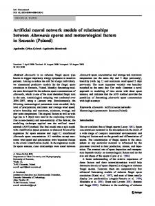
An important question addressed in this paper refers to the role played by the activity of the examples, a, on the categorization ability of the network. In Fig. 2 the categorization error εc is shown as a function of the activity, for α = 0.02, s = 20, b = 0.2 and for several values of θ. The results reveal that εc is a monotonically increasing function of a. Since this is the general behavior for other values of the parameters, the results confirm that for the connected, as well as for the dilute [19] networks, it is better to train the network with low-activity examples. This can be understood noting that the activity a of the examples is decreased when a macroscopic number of bits of every example is turned off. But in keeping the overlap b between examples and concepts fixed, the bits that are turned off in the examples must be those that are inverted with respect to the concepts . When the activity a reaches its minimal, optimal value, a = b, the only bits that are turned on in the examples are those that are aligned with the concepts, leading to the smallest categorization error. In this case the categorization task of the network becomes similar to the reconstruction of a puzzle from loose pieces. Finally, the figure also shows the discontinuous jump to the spin-glass (SG) phase, at the upper phase boundary of Fig. 1. The categorization error as a function of the number of examples s, for b = 0.4, θ = 0 and θ = 1.0 and two different activities, namely a = b (all wrong bits in the examples are turned off) and a = 1.0 (all wrong bits in the examples are included) is shown in Fig. 3. Starting from the spin glass phase, with categorization error equal to 0.5, the network undergoes a discontinuous transition to the categorization phase as the number of examples increases above a critical value. The number of examples required for the jump to the categorization phase is considerable smaller for a = 0.4, than for a = 1.0. Nevertheless, the final categorization error is similar for the two activities. This means that the network is able to overcome a higher amount of errors in the examples by a larger number of these examples. A higher value of s is also required for a higher threshold θ, in order to reach a higher local field to attain the states with non-zero activity.

13

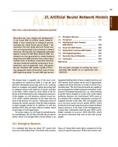
B. Categorization properties in the presence of synaptic noise We consider next the categorization performance obtained from Sβ (hs , θ ′ ), Eq. (43), for finite β. Fig. 4 illustrates the influence of the temperature on the categorization error, for α = 0.01, s = 20, b = 0.2 = θ, and activity a equal to 0.2 and 0.3. To the left of the arrow in the curve corresponding to a = 0.2, the categorization phase is the global minimum, while it is a local minimum to the right. In what concerns the present set of parameters, the categorization phase for a = 0.3 is a local minimum for all temperatures, whereas the spin-glass phase is the global minimum. Thus, it is also advantageous for an enhancement of the performance of the network, in the presence of synaptic noise, to train the network with examples of low activity. Fig. 4 also shows the discontinuous transition to the spin-glass phase at an activity-dependent transition temperature. The phase diagram for α vs. T is presented in Fig. 5 for θ = 0.2, s = 20 and a = 0.2 = b. The categorization phase is stable below the upper phase boundary, where it disappears discontinuously, becoming a global minimum below the lower phase boundary. At very small α and T there is a retrieval phase without categorization, not shown in the figure. The dashed line on the left is the locus of the AT-line. The replica-symmetric solution for the categorization phase becomes unstable to replica-symmetry-breaking fluctuations at the left of this line. The re-entrant behavior of the upper phase boundary at low T is associated to the instability of the replica-symmetric solution in this region. The spin-glass phase becomes a global minimum to the right of the heavy solid, and to the left of the dotted line, where it disappears continuously. At the right of the dotted line, the paramagnetic phase is the global minimum.

V. NETWORK WITH CONTINUOUS NEURONS

In this section we discuss the categorization properties of a network with continuous, monotonic neurons trained with continuous or discrete examples of binary concepts. The continuous limit is obtained by taking Q → ∞ in Eqs. (1) and (15). The following results are independent of the specific form of P (λµρ i ), provided that its mean and variance are given by Eqs. (3) and (4),

14

respectively. The general Eqs. (39)-(42), for the saddle-points, apply also to this case. In the absence of noise, the effective transfer function, Eq. (44), becomes the stepwise linear function S∞

h h min h, θ = sign 2θ ′ , 1 2θ ′ 

′










,

(54)

in which 1/2θ ′ is the effective gain parameter. Consequently we obtain 1 1 sms b sms b m1 = erf (M− ) + erf (M+ ) 1− 1+ ′ 2 2θ 2 2θ ′ r    i 1 v h − ′ exp −M−2 − exp −M+2 , 2θ 2π 



q =1−





(55)

h    i v 2 2 √ M exp −M − M exp −M + − − + 4θ ′2 π

"

v 1 + 1 + ′2 2 2θ

1 s2 m2s b2 + 2 2v

!#

[erf (M− ) − erf (M+ )]

(56)

and C=

1 [erf (M+ ) − erf (M− )] , 4θ ′

(57)

where M± =

sms b ± 2θ ′ √ . 2v

(58)

The zero-temperature phase diagram for α vs. θ with s = 20 and a = 0.2 = b is shown in Fig. 6. The categorization phase exists below the light solid line, and it is the global minimum below the heavy solid line. At the left of the dotted line, θ ′ is zero and the effective gain is infinite. In this region, the states Si = ±1 are the only accessible states for non-zero local field and the network behaves as a binary network. In there, the critical α for categorization assumes its value in the binary network for this set of parameters, i. e., αc,binary ≈ 0.033. When the network enters the multi-state, continuous regime, the categorization capacity starts to increase abruptly, and reaches its maximum value αc ≈ 0.047 for θ ≈ 0.11. The dashed line signals the optimum θ for each α. It is worth noting that for α < αc,binary the optimal θ line coincides with the transition to the binary regime. This means that whenever there is a binary network capable to perform the categorization task, it will give the best categorization properties for low θ. Only when α > αc,binary the network

15

with continuous neurons is expected to have a better performance. Contrary to the case of finite Q, where at zero temperature the replica-symmetric solution is always unstable, there is here a region where it is stable, and this is the part of the phase diagram below the light dash-dotted line. The phase diagram illustrates that also the network of continuous neurons is robust to low gain in the states. The existence of a replica-symmetric stable phase at zero temperature was noticed in ref. [8], for the retrieval problem in a network of continuous neurons. Finally, the heavy dash-dotted line represents the onset of the continuous spin glass transition. In Fig. 7 we present the categorization error as a function of the activity of examples, for α = 0.02, s = 20, and θ = 0.2 to 0.4. Since we deal with a non specified P (λµρ i ), the only restriction imposed is a ≥ b2 . We note from the figure that the categorization error is no longer a monotonic increasing function of the activity for all values of θ. For θ = 0.4, εc is a decreasing function of a, for small a. The reason is that in the case of large threshold θ, the local field hi ({Si }) must be sufficiently high to overcome the threshold, and this is obtained through a moderate increase in the activity of the examples. Finally, we discuss the influence of the number of examples s on the categorization ability of networks with continuous neurons. Fig. 8 shows the categorization error as a function of s for a = 0.2 = b, threshold ranging from 0.2 to 0.4 and α = 0.02. As a result of the continuous nature of the units, for low threshold the categorization error decreases smoothly with the increasing number of examples. This is distinct to the previous case of discrete units, where an abrupt decrease in εc was observed even at θ = 0 (see Fig. 1). Furthermore, the decreasing in εc is no longer monotonic for all values of the threshold. For example, for θ = 0.2 there is a local maximum in εc for s ≈ 30.

VI. SUMMARY AND CONCLUDING REMARKS

The categorization problem, that consists of the recognition of ancestors, when a network is trained only with their descendents, is studied in this work for multi-state fully connected neural network models, keeping in mind an application to either artificial or biological networks in which the training is with sparsely coded patterns. Indeed, multi-state networks offer the possibility of

16

recognizing full-sized patterns in networks trained with “small” patterns, in which a macroscopic number of bits have been reduced or, eventually, set to zero reducing thereby the activity of the encoded patterns. We found that a low activity can enhance the categorization ability of a fully connected network in a significant way, by changing the threshold for firing of the units. This confirms and extends earlier results on an extremely dilute network of Q = 3-state neurons [18]. The way the network works for the categorization task is the following. After training with correlated examples, the network searches for stable symmetric mixtures states, in place of pure examples. If these patterns have low activity, it will be less likely that they have bits with opposite sign to the corresponding concepts. The recognition of the latter from the common features of the examples will thereby be enhanced. We derived formal expressions, within replica-symmetric mean-field theory, for the free energy and the relevant order parameters for the categorization problem in a fully connected neural network model, with units in general Q Ising-states and multi-state patterns belonging to a two-level hierarchy. Training of the network was assumed to take place through a generalized Hebbian learning rule involving only the descendents. These may be considered as corrupted examples of the ancestors (concepts) with a number of turned off or inverted bits. Explicit results for the relevant phase diagrams and the categorization curves were then obtained for a Q = 3-state model with a monotonic activation function and for a monotonic Q = ∞-state model. In the first case we also checked the robustness of the network performance to synaptic noise. Our results are restricted to binary ancestors and multi-state descendents, although the case of multi-state ancestors has been considered in an extremely dilute network [21]. The limit of validity of the replica-symmetric solution was established in this work looking for the Almeida-Thouless lines. For Q = 3, the replica-symmetric solution is unstable in the absence of synaptic noise (T = 0) and there is a re-entrant behavior for the ratio α of recognized concepts, at small synaptic noise, in accordance with earlier results on the retrieval problem [37,38] and on the categorization problem in connected networks of binary neurons [31]. Nevertheless, since the replica-symmetric solution stabilizes at very small T , we argue that replica-symmetry breaking effects should be negligible, even at T = 0. On the other hand, there is a finite region of interest

17

for the categorization performance domain where the replica-symmetric solution is stable, even at T = 0, in the case of the Q = ∞-state network, as demonstrated explicitly in this work. To summarize, we succeeded in studying a fully connected multi-state neural network model for the categorization problem of recognizing binary concepts when the network is trained with Q-state examples of low activity, in place of the full activity patterns of a binary network of states S = ±1. The work presented here can be extended in various directions. First, to infer multistate concepts in a network with full connectivity and to study the categorization performance for sparsely coded sequential examples. In order to come closer to biological networks, it would be interesting to consider the partial dilution of synapses. Acknowledgments We are indebted to Alba Theumann for showing us how to find the Almeida-Thouless line for a network with hierarchically correlated patterns. We thank D. Boll´e for comments and discussions, as well as for the kind hospitality of the Institute for Theoretical Physics of the Catholic University of Leuven, where part of the work of DRCD and WKT was done. This work was supported, in part, by CNPq (Conselho Nacional de Desenvolvimento Cient´ıfico e Tecnol´ ogico, Brazil), and FINEP (Financiadora de Estudos e Projetos, Brazil).

18

REFERENCES [1] J. Hertz, A. Krogh and R. Palmer, Introduction to the Theory of Neural Computation (Reading, MA: Addison-Wesley, 1991). [2] J. S. Yedidia, J.Phys. A: Math. Gen. 22, 2265 (1989). [3] C. Meunier, D. Hansel and A. Verga, J. Stat. Phys 55 859 (1989). [4] H. Rieger, J. Phys. A: Math. Gen. 23, L1273 (1990). [5] S. Mertens, H. M. K¨ ohler and S. B¨os, J. Phys. A: Math. Gen. 24, 4941 (1991). [6] G. A. Kohring, J. Physique 2, 1549 (1992); Neural Networks 6, 573 (1993). [7] M. Bouten, and A. Engel, Phys. Rev. E 47, 1397 (1993). [8] D. Boll´e, H. Rieger, G. M. Shim, J. Phys. A: Math. Gen. 27, 3411 (1994). [9] R. K¨ uhn and S. B¨os, J. Phys. A: Math. Gen. 26, 831 (1993). [10] D. Boll´e and J. Huyghebaert, Phys. Rev. E 52, 870 (1995). [11] D. Boll´e, J. L. van Hemmen and J. Huyghebaert, Phys. Rev. E 53, 1276 (1996). [12] D. Boll´e and R. Erichsen Jr., J. Phys. A: Math. Gen. 29, 2299 (1996). [13] R. Erichsen Jr. and W. K. Theumann, Phys. Rev. E 59, 947 (1999). [14] D. Boll´e and R. Erichsen Jr., Phys. Rev. E 59, 3386 (1999). [15] C. M. Marcus, F. R. Waugh, and R. M. Westervelt, Phys. Rev. A 41, 3355 (1990). [16] D. Boll´e, B. Vinck, and V. A. Zagrebnov, J. Stat. Phys. 70, 1099 (1993). [17] D. A. Stariolo and F. A. Tamarit, Phys. Rev. A 46, 5249 (1992). [18] D. R. C. Dominguez and W. K. Theumann J. Phys. A: Math. Gen. 29, 749 (1996). [19] D. R. C. Dominguez and W. K. Theumann, J. Phys. A: Math. Gen. 30, 1403 (1997).

19

[20] D. R. C. Dominguez, Phys. Rev. E 54, 4066 (1996). [21] D. R. C. Dominguez and D. Boll´e, Phys. Rev. E 56 7306 (1997). [22] J. F. Fontanari and R. Meir, Phys. Rev. A 40, 2806 (1989). [23] J. F. Fontanari, J. Physique 51, 2421 (1990). [24] E. Miranda, J. Phys. I France 1, 999 (1991). [25] M. C. Branchstein and J. J. Arenzon, J. Phys. I France 2, 2019 (1992). [26] P. R. Krebs and W. K. Theumann, J. Phys. A: Math. Gen. 26, 398 (1993). [27] R.Crisogono, A.Tamarit, N.Lemke, J.Arenzon and E.Curado, J. Phys. A: Math. Gen. 28, 1593 (1995). [28] C. Rodrigues Neto and J. F. Fontanari, J. Phys. A 31, 531 (1998). [29] J. A. Martins and W. K. Theumann, Physica A 253, 38 (1998). [30] R. L. Costa and A. Theumann, Physica A, to be published. [31] P. R. Krebs and W. K. Theumann Phys. Rev. E, to be published. [32] N. Parga and M. A. Virasoro, J. Phys. A: Math. Gen. 47, 1857 (1986). [33] H. Gutfreund, Phys. Rev. A 37, 570 (1988) [34] B. Derrida, E. Gardner, and A. Zippelius, Europhys. Lett. 4, 167 (1987). [35] M. A. P. Idiart and A. Theumann, J. Phys. A: Math. Gen. 25, 779 (1992). [36] J. R. de Almeida and D. Thouless, J. Phys. A: Math. Gen. 11 983 (1978). [37] A. Canning and J.-P. Naef, J. Phys. I France 2, 1791 (1992). [38] J.-P. Naef and A. Cunning, J. Phys. I France 2, 247 (1992).

20

FIGURES FIG. 1. Phase diagram for the ratio α of recognized concepts as a function of the threshold θ, for the three-state network. The number of examples is s = 20, the activity a = 0.2 = b (the correlation parameter). Here, C, SG and P are the categorization, spin-glass and paramagnetic phases, respectively. Below the heavy solid line, the categorization phase is the absolute minimum of the free-energy. Solid (dash-dotted) lines indicate a discontinuous (continuous) transition. The dashed line indicates the optimal value of θ. At the left of the dotted line, the network behaves as a binary network with states Si = ±1. FIG. 2. Categorization error as a function of the activity a, for the three-state network at T = 0, when α = 0.02, s = 20, b=0.2 and θ = 0.0–0.3 (as indicated). FIG. 3. Categorization error as a function of the number of examples s, for the three-state network at T = 0, when α = 0.05, b = 0.4. Solid (dotted) lines correspond to θ = 0.0 (θ = 1.0) and the two lines at the left (right) correspond to a = 0.4 (a = 1.0). FIG. 4. Categorization error as a function of the temperature T , for the three-state network, when α = 0.01, s = 20, b = 0.2 = θ and a = 0.2 (solid line) and 0.3 (dotted line). FIG. 5. Categorization phase diagram of α vs. T , for the three-state network, when θ = 0.2, s = 20 and a = 0.2 = b. Below the heavy solid line the categorization phase is the absolute minimum of the free energy. Solid (dotted) lines indicate a discontinuous (continuous) transition. The replica symmetry is broken at the left of the dashed line.

21

FIG. 6. Categorization phase diagram of α vs. θ, for the continuous Q = ∞-state network, at T = 0, when s = 20, a = 0.2 = b. Here, C, SG and P are the categorization, spin-glass and paramagnetic phases, respectively. Below the heavy solid line the categorization phase is the absolute minimum of the free-energy. Solid (heavy dash-dotted) lines indicate discontinuous (continuous) transitions. The dashed line indicates the optimal value of θ. At the left of the dotted line, the network behaves as a binary network with states Si = ±1. Below the light dash-dotted line the replica symmetric solution is stable. FIG. 7. Categorization error as a function of the activity a, for the Q = ∞-state network at T = 0, when α = 0.02, s = 20 and b=0.2. The threshold values are 0.2, 0.3 and 0.4 (curves from right to left). FIG. 8. Categorization error as a function of the number of examples s, for the Q = ∞-state network at T = 0, when α = 0.02 and a = 0.2 = b. The threshold values are 0.2, 0.3 and 0.4 (curves from left to right).

22

0.04

SG

0.03

α

SG,C 0.02

P 0.01 C,SG

0.00 0.0

0.2

θ

0.4

0.6

0.6

0.4 0.2

0.3

0.1

εc

0.2 0.0

0.0 0.20

0.22

0.24

0.26

a

0.28

0.30

0.6

0.4

εc

0.2

0.0

0

20

40

60

s

80

100

0.6

0.4

εc

0.2

0.0 0.0

0.2

T

0.4

0.04

0.03

SG

α

0.02 SG,C

0.01 P

C,SG

0.00 0.0

0.2

0.4

T

0.6

0.8

0.06

SG

0.04

SG,C

α

0.02

P C,SG

0.00 0.0

0.2

0.4

θ

0.6

0.8

0.6

0.4

εc

0.2

0.0 0.0

0.2

0.4

a

0.6

0.4

εc

0.2

0.0

0

20

40

s

60

80