Holographic implementation of a fully connected neural network ...

Holographic Implementation of a Fully Connected Neural Network KEN-YUH HSU, HSIN-YU LI,

AND

DEMETRI

Invited Paper

This paper describes an optical implementation o f a fully connected neural network similar to the Hopfield network. Experimental results which demonstrate i t s ability to recognize stored images are given, followed b y a discussion o f its performance a n d analysis based on a proposed model for the system.

I.

.

INTRODUCTION

In this paper we present a holographic implementation of a fully connected neural network [I], [2]. This model has a simple structure and i s relatively easy to implement while its operating principles and characteristics can be extended to other types of networks, since any architecture can be considered as a fully connected network with some of i t s connections missing. In the following sections, the basic principlesof the fully connected networkare reviewed.The optical implementation of the network is presented in Section Ill and itsexperimental results are presented in Section IV. Special attention i s focused on the dynamics of the feedback loop and the trade-off between distortion tolerance and image-recognition capability of the associative memory. Mathematical modeling and analysis of the system are presented in Section V.

~kC0IlXleCtbM

Ncumar

Fig. 1. Two dimensional fully connected network.

There are two phases in the operation of the network: learning and recall. In the learning phase, the information to be stored i s recorded according to the outer product scheme [I], [2]. This storage specifies the interconnection strengths between the neurons. In the recall phase, an external input i s presented to the system. The state of the system then evolves according to the correlation between the input and the stored data. M N-bit binary words are stored in a matrix w,,,according to

II. THE HOPFIELD MEMORY

/ M

The basic structure of the network i s shown in Fig. 1. It i s a single-layer network with feedback. There are two main components: the neurons and the interconnections. The neurons are distributed in the neural plane. The neurons receive inputs, perform nonlinear thresholding on the received input, provide gain, and re-emit the output patterns. The output of each unit i s connected to the input of all other neurons to form a feedback network. Manuscript received September 25,1989; revised April 12,1990. Thiswork issupported by DARPAand i n part by the Air Forceoffice of Scientific Research. K.-Y. H s u waswith the Department of Electrical Engineering, California Institute of Technology, Pasadena, CA 91125, USA. He i s now with the Institute of Electro-Optical Engineering, National Chiao Tung University, Hsin-Chu 30050, Taiwan, ROC. H.-Y. Li and D. Psaltis are with the Department of Electrical Engineering, California Institute of Technology, Pasadena, CA 91125, USA. IEEE Log Number 9039181.

otherwise, where vT = + I , i = 1, . . . , N, i s the i t h bit of the moth memory. Suppose, for example, that vmo, the mth stored vector, i s presented to the system in the recall phase. This vector i s multiplied by the matrix w,,,,giving the output of the first iteration:

vo= sgn [jl w,,,v:..],

(2)

where sgn{ . } i s the thresholding function, sgn{x}

1, =

-1,

if x

2

0;

i f x < 0.

(3)

The thresholded result of the first iteration is then fed back to the system as input for the next iteration, and so on.

0018-9219/90/1000-1637$01.00 0 1990 IEEE

PROCEEDINGS OF THE IEEE, VOL. 78, NO. IO, OCTOBER 1990

Authorized licensed use limited to: EPFL LAUSANNE. Downloaded on August 27, 2009 at 11:24 from IEEE Xplore. Restrictions apply.

1637

There are three operations performed by the system: vector-matrix multiplication, thresholding? and feedback. A network of this type using optoelectronics was first implemented by Psaltis, Farhat, and their colleagues [3], [4]. They used a computer-generated transparency to provide the interconnection matrix. A I - D array of 32 photodiode pairs followed by electronic thresholding plus a I - D array of 32 LEDs was used to simulate 32 neurons. In this paper the optical implementation of such a system for2-D images uses holograms. The design and implementation of this system are presented in the following section. Ill. OPTICAL IMPLEMENTATION

M

,,,?, frn(x, y)frn(t, v),

(4)

where f,,,(x, y ) i s the mth image, and M i s the total number of images to be stored. Note that o ( x , y; F , 7) i s a four dimensional kernel and cannot be implemented directly using a single transparency since a 2-D optical system has onlytwo spatial coordinates. The system described in this paper i s based on a method for implementing this 4 D kernel that uses a 2-D array of spatial frequency multiplexed holograms [3], [SI, [6]. Janget al. used a 2-D array of N x N diffused holograms to obtain the 4-D interconnection [7J, [SI. Other approaches to this problem include the use of spatial multiplexing [9] and volume holograms [101-[13]. In the recall phase, the output of the system is described by the equation

f(x, y, t ) = g

[11

W(x, y; t , ~

Pl

optical loop.

The interconnection pattern for 2-D images i s described by the following equation:

~ ( xY;, F , 7) =

"SzSztmd

Fig. 2. Block diagram of the operations performed by the

t7, w,t Q j .

(5)

where g{ represents the nonlinear thresholding of the neurons, f ( x , yf t) i s the input to the system at time t, and ?(x, y, t ) i s the output of the system. Substituting the expression for o ( x , y; t , 7) into this equation, and rearranging the order of integration and summation, we obtain

betweenthe input and each of the stored imagesform. Each of the four signalsthat pass through thepinholesactasdelta functions, reconstructing from the second correlator the four images that are stored there. These reconstructed images are spatially translated according to the position of each pinhole and superimposed at plane f,. At the center of the output plane of the second correlator we obtain the superposition of the four stored images. The stored image that is most similar to the input pattern gives the strongest correlation signal, hence the brightest reconstructed image. In Fig. 2 we show only the image that i s reconstructed by the strongest auto-correlation peak. The weak read-out signal that is due to cross-correlations is suppressed by the thresholding operation of the neurons. The output from the plane of neurons becomes the new input image for the next iteration. In this way the stable pattern that i s established in the loop i s typically the stored image that is most similar to the original input. The optical implementation makes use of the Vander Lugt correlator [I41shown in Fig. 3. If we place a hologram at the

e }

?(x, yt t) = g

*

[jl [ 1 1 frn(xt y )

f(t - x,

7

frn(tt

- y, OdFd?]

1.

output

Fig. 3. Vander Lugt correlator.

(6)

From (6)we see that the implementation of the 2-D associative memory can be achieved in three steps [6]. First the 2-D correlation between the input image f and each of the memories f,,, i s calculated, and then the correlation function i s evaluated at the origin to obtain the inner product values. Second, each inner product i s multiplied by the associated stored memory. Third, these products are summed over all memories and thresholded by the neurons. The implementation of the system will be explained with the aid of Fig. 2. Here four images are spatially separated and stored as the reference images in each of two correlators. When one of the stored patterns A i s presented at plane Pl of the system, the first correlator producesthe autocorrelation along with three cross-correlationsof plane Pz. The pinhole array at f 2samples these correlation functions at the center of each pattern where the inner products

1638

Fourlar

.. ./

7)

x = 0,y = 0

Input pkne

Fourier plane of the system in Fig. 3 whose transmittance function i s the complex conjugate of the Fourier transform of a second, reference image, then it can be shown that the output is the 2-D correlation function between the input and reference images [151. In our system, the reference image in each of two correlators i s a composite of four images that are spatially separated. A transparency i s prepared containingthe four images and the Fourier transform of this pattern i s formed with a lens. A hologram of the Fourier transform of the composite pattern i s then formed by recording its interference with a plane wave reference. The hologramsthat are formed in this manner are placed at the intermediate planes of two Vander Lugt correlators that are cascaded to form the optical memory loop. The schematic diagram of the overall optical architecture i s shown in Fig. 4, and a photograph of the experimental apparatus is shown in Fig. 5. The first correlator consists of the liquid crystal light valve (LCLV) at fl, the beam splitter

PROCEEDINGS OF THE IEEE, VOL. 78, NO. 10, OCTOBER 1990


Argon IAaer

Fig. 4.

LCLV

Bsg

L,

Input

Schematic diagram of the optical loop.

(b)

(C)

Fig. 6. Stored images. (a) The original images. (b) Images reconstructed from H , . (c) Images reconstructed from H,.

Fig. 5.

.

Photograph of the optical loop.

cube BS,, the lenses L,, L,, and the hologram H,. The LCLV here functions as a 2-D array of neurons. It consists of a dielectric mirror sandwiched between a light-sensing layer and a light-modulation layer. The light-sensing layer i s a CdS photoconductor which acts as a photosensor, whereas the light-modulation layer is a thin layer (a few microns) of nematic liquid crystal. When light strikes the photosensor, itsconductancechanges,which in turn changesthevoltage across the liquid crystal on the other side. When a reading light beam across the liquid crystal layer i s reflected off the light-modulatingside, its polarization state i s modulated in proportion to the voltage across the liquid crystal layer. The second correlator consists of P,, L3, H,, L4, BS3, and P, shown in Fig.4.The input pattern is imaged ontothe LCLV by lens L, and through beam splitter 6S3. A collimated argon laser beam illuminates the read-out side of the LCLV through beam splitters BS, and BS,. A portion of the reflected light from the LCLV that propagates straight through BSI, i s diverted by BS,, and it i s imaged by lens Lo onto a CCD television camera through which we monitor the system. The portion of light reflected by BS, into the loop i s Fourier transformed by lens L, and illuminates hologram HI. The correlation between the input image and each of the stored images i s produced at plane P2.The spacing of the pinhole array at P2 correspondst o the spatial separation between the stored images. The remainder of the optical system from P2 back t o the neural plane P1 i s essentially a replica of the first half, with hologram H2storing the same set of images as H,. The holograms in this system are thermoplastic plates, with an area of 1 in2and 800 linedmm resolution. The hologram H1 i s made with a high-pass characteristic for edge enhancement t o improve discrimination. H, on the other hand i s broadband so that the feedback images have high fidelity with respect to the originals. We use a diffuser t o

achieve this when making HZ.Fig. 6(a) shows the four original images. Fig. 6(b) shows the images reconstructed from the first hologram H1,and Fig. 6(c) shows the images reconstructed from the second hologram H,. The pinhole array at P, samples the correlation signal between the image coming from the LCLV and the images stored in hologram H,. The pinhole diameter used in these experiments ranges from 45 pn to 700 pm. If the pinholes are too small, the light passing through to reconstruct the feedback image is too weak to be detected by the LCLV. On the other hand, large pinholes introduce excessive blurring and cross-talk and make the reconstructed images unrecognizable. The pinhole size also affects the shift invariance of the loop. I n order to be recognized, the autocorrelation peak from an external image should stay within the pinhole. Larger pinholes allow more shift in the input image. The system performance under different selections of pinhole diameters i s discussed in the next section. As the optical signal goes through the loop, it i s attenuated because of the small diffraction efficiency of the Fourier transform holograms and the losses from pinholes, lenses, and beam splitters. To compensate for this loss, we use an image intensifier at the photoconductor side of the LCLV. The microchannel plate of the image intensifier is sensitive to a minimum incident intensity of approximately 1 nW/cm2 and reproduces the input with an intensity IO4 times brighter (IO pW/cm2),sufficient t o drive the LCLV. If we use a beam with intensity equal to 10 mW/cm2to read the LCLV, then the intensityof theoutput light i s approximately1 mW/ cm2.Thus, the combination of the image intensifier and the LCLV provides an optical gain up to IO6. It turns out that the setting of the gain is the key parameter that mediates the trade-off between distortion invariance and the discrimination capability of the loop. This will also be discussed in the next section. IV. EXPERIMENTAL RESULTS The optical associative loop of Fig. 4 can be lumped into the simplified blocks shown in Fig. 7(a). The LCLV i s represented as the component Gain i n Fig. 7(a). The other parts of the loop are all lossy, linear components and are represented by the component Loss in Fig. 7(a).

HSU et al.: HOLOGRAPHIC IMPLEMENTATION OF A FULLY CONNECTED NEURAL NETWORK


1639

* j r a

Qdn

Input

Output

*

t

t3

(b) Fig. 7. (a)The gain and loss components of the loop. (b)The

stable states of the loop.

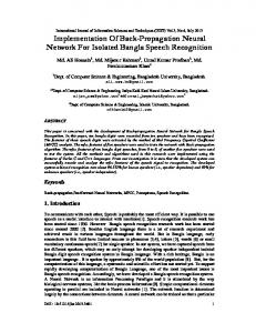
The dynamics of the recall process can be understood by using the iteration map shown in Fig. 7(b). In the figure the gain curve represents the input-output response of the neurons, whereas the straight line gives the loop l o ss due to the holograms, and pinholes, etc. The intersection point Q1i s the threshold level, and the intersection point Q2gives a stable point. If the initial condition is above the threshold level e,, the signal (I,) grows in successive iterations until it arrives and latches at Q2. O n the other hand, if the initial condition i s belowo,, thesignal (/,)decaystozero.The number of iterations (convergence time) depends on the initial condition.Thisof course isonlya simplified pictureof what goes on in the loop. A more precise analysis will be given in Section V. The loopdynamicswere measured by controllingthetwo shutters shown in Fig. 7(a). An example of the temporal response of the loop to an input pattern i s shown in Fig. 8. The lower trace represents the intensity of the external input image and the upper trace represents the corresponding light intensity detected at the loop output. Before time tl, both shutters are closed and the response i s low. At time tl the input shutter i s opened (with the loop shutter still closed) and the lower trace becomes high. The upper trace shows the corresponding response of the neurons to the external input. At time f2 the loop shutter i s opened and the loop i s closed. The feedback signal arrives at the neurons as an additional input and iteration begins. It takes about two seconds in this case for the loop to reach a stable state. At time t3 the input shutter i s closed and the lower trace becomes low. However, the loop remains latched to a stable state, which i s one of the stored images. We get similar resultswith reduced input intensity. It takes longer to reach a stable state when the input i s weak, but the final state remains the same. Since the external input does not affect the shape of the final state, but only selects which state i s produced, there i s a certain degree of invariance in the system since a distorted version of a stored image can recall the stored image. The effect of distortions such as scale, rotation and shift,

t

t

Fig. 8. Temporal response of the loop. (a) Strong input. (b) Weak input. Timing: t, = Input ON, f L = Feedback ON, t 3 = Input OFF.

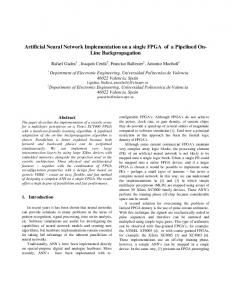
is todecrease the initial intensity level of the loop. However, as long as the initial condition is above the threshold (6' in Fig. 7(b)), the loop still converges to a memory state. The strength of the initial condition is determined bythedegree of distortion of the input,whilethe threshold isdetermined by the neural gain and loop loss. The images stored in the loop are the four faces shown in Fig. 6(a). Fig. 9(a) shows the response of the system when a partially blocked face i s presented to the system with the loop shutter closed. This sets the initial condition. The loop shutter i s then opened to close the feedback path, and the stateof the system evolves.After some time the loop reaches stable state and a complete face appears. The time for this process ranges from less than one second to several seconds, depending on the initial condition and the system parameters. The complete image remains latched in the loop when the external input is removed. Fig. 9(b) shows the system output at the moment the loop shutter is closed. We see that the feedback image i s superimposed on the input. Fig. 9(c) to (e) shows the evolution of the output after the feedback loop i s closed. The complete image obtained 2 seconds after the loop is closed i s shown in Fig. 9(e). Fig. 9(f) shows that after the external input is removed, the recalled image stays latched. The same situation occurs when other partially blocked faces are used. In a separate experiment, a rotated version of each of the faces was used as input. Fig. 10(a) shows the output of the

PROCEEDINGS OF T H E IEEE, VOL. 78, NO. IO, O C T O B E R 1990

1640

.


I

(e) Fig. 9. Retrieval of the complete image from the partial input. (a) The partial input at t = 0. (b) t = 0' (loop closed). (c) t = 400 ms. (d) t = 800 ms. (e) t = 2 sec. (f) Input OFF.

loo lbo goo dw mft (4 (b) Fig. 11. (a) Loop response to rotated inputs. (b) Loop response to shifted inputs. (Optical gain = lo4; 0:Output intensity. U: Loop rise time.)

(e)

(f )

Fig. 10. Retrieval of the complete image from the rotated input. (a) The input at t = 0. (b) t = O + (loop closed). (c) t = 1.8 sec. (d) t = 3.6 sec. (e) t = 4.8 sec. ( f ) Input OFF.

system when a rotated version (by 6") of one of the faces i s presented to the system with the loop shutter closed. Fig. 10(b)shows the memory output immediately after the feedback loop i s closed. The evolution of the system towards the original unrotated image i s shown in Fig. 1O(c) to Fig. 10(e). In Fig. 1l(a) the upper curve is the intensity of the final image and the lower curve i s the convergence time, both plotted as functions of rotation angle. The larger the rotation angle, the longer it takes to converge. However, once the loop reaches stable state, the output intensity i s always the same regardless of the initial rotation. The output intensitydropstozerowhen theangle i s morethan8O.This means that the initial condition i s below threshold and the rotated image does not elicit a response. One way to increase tolerance to rotation i s by increasing the neural gain SO that it can detect weaker feedback signals. It i s found that with the gain set 10 times higher, the tolerance increases to 16".

HSU et

a/

However, although we can obtain more tolerance by increasing the gain, this enhances crosstalk and may cause the loop to converge to the wrong image. Similar experiments were carried out to measure the ability of the system to tolerate scale changes. The results were similar, with tolerance in the range of 7% to 9%, depending on the gain. This system has very small tolerance to position errors at the input, i.e., it i s not shift invariant. When the input image is translated, the entire correlation pattern in the intermediate plane P2 shifts also. The autocorrelation peak that is normally aligned with the pinhole i s blocked. A small degree of shift invariance exists due to the finite width of the pinhole and the correlation peak. In the experimental system, the pinhole diameter was 90 pm. Fig. I l ( b ) shows the strength of the final state and the rise time versus the amount of shift in the input from i t s nominal position. A larger pinhole yields more shift invariance. But as the pinhole diameter increases, the reconstruction from the second hologram i s blurred because the output becomes the convolution of the stored image with its autocorrelation pattern. This results in a l o s s in correlation strength in subsequent iterations, and can result in insufficient gain for maintaining a stable state. The experimental results shown above demonstrate the distortion-invariance capability of the associative loop. By raising the neural gain sufficiently high, the loopcan always be made to produce an image as a stable state no matter how much wedistort the input image. But the ability to reliably produce correct associations between initial and final states degrades as the gain increases. If there i s too much gain, then just shining a flashlight at the input of the system can cause it to converge to one of its stable states. I f the gain i s set too low, the slightest distortion of the stored images renders it unrecognizable. If the gain i s set even lower, no input can cause the loop to latch on a stable state. Fig. 12

HOLOGRAPHIC IMPLEMENTATION OF A FULLY CONNECTED NEURAL NETWORK

__

-


1641

optics i s M

wij =

C (xy m=l

- a,,,)xy,

(7)

where a,, = 1 / N CYz1x,"' i s the mean value of the mth memory.Aneuron isoptically simulated byone pixelof theLCLV, which i s modeled as shown in Fig. 13. Let xi denote the out-

output

Input /

..

---.

\

/ Fig. 12. Loopdynamics with high optical gain. (a)The input at t = 0. (b) t = O + (loop closed). (c) t = 1.2 sec. (d) t = 1.8 sec. (e) The input i s OFF. (f) Stable state.

\

/ Y

*+, I

I

I

\

shows an example of the behavior obtained when the gain is set too high. An unfamiliar input initially produces an unrecognizable state. When the external input i s removed, the system latches erroneously to one of the stored images.

\

/ Optical Neuron

Fig. 13. Model for the LCLV and the gain function.

v.

A NETWORK MODEL FOR

THE

OPTICAL LOOP

The optical associative memory presented in this paper i s very similar to a Hopfield network, but it is not quite the same. The neurons are simulated by the LCLV, which responds to light intensity, which i s the magnitude squared of the light amplitude, the quantitythat is modulated bythe output stage of the LCLV and multiplied by the weights. Consequently, the input signal to the neurons is first squared before beingthresholdedand as a result the neural gain i s unipolar instead of bipolar(as in the Hopfield model). The interconnection weights are bipolar quantities (actually they can be complex since they are holographic gratings), As mentioned before, the first correlator contains a high pass version of the stored memories. In our analysiswe will assume that the high pass filtering operation subtracts the mean value of each image, thus transforming the unipolar initial images into their bipolarversions. Since in theoptical system the outer product needed to specify the interconnection matrix i s formed as acascadeoftwo correlators, the resulting weight i s the outer product between bipolar and unipolar versions of the stored images. These differences give us characteristics that are distinct from the Hopfield model, such as a ground state (which the Hopfield model does not have) and a dependenceof the stable states on the gain the system (in the optical system an increase in gain transforms the shape of the stable states). Thus although the Hopfield model has been analyzed extensively, all the results can not be applied directly to our system, and further analysis i s necessary. In the following, we present a model for the optical associative-memory loop described above. For simplicitywe will revert in the subsequent analysis to I-D, discrete notation. Let x y denote the i-th bit of the mth unipolar (0 or 1) memory. The interconnection matrix that i s implemented by the

1642

put of the i t h neuron (or equivalently the reflectivity of a pixel on the LCLV). Then

where g i s a nonlinear function describing the neuron response. Note that g is an even function instead of an odd (sigmoid-like) function, as is usually assumed. In the above equation the response of each pixel i s coupled to all other pixels and depends on all the memories stored in wq.To gain some understanding about what the stable states are and how they are related to the patterns we attempt to store in the system, we introduce a change of variables. ,!?'are linearly Assumethat the stored imagesxl,xZ, * independent. We decompose the vector space RN into two subspaces, V,and V,,where V, i s the vector space spanned by the stored images and V, is normal to V,. We define a basis p1 = { y ' , y z , . . ,y M } for V,,such that yi

x i = 6,

i , j = 1,

... ,M

(9)

and we select an orthonormal basis p2 = { y M + l , * , y"} ,y N } which for V,. We then have p = U p2 = { y ' , forms a basis for R". Consider the vector U whose j t h component i s (xI - I/ NC;=,xk). (We will call U the bipolar version of x.) Let cI be the I t h component of U expanded in terms of the basis 0. Using (g), a set of differential equations can be found for the cis:

PROCEEDINGS OF THE IEEE, VOL. 78, NO. IO, OCTOBER 1990

3 = dt

-cf

+

In this case, the driving forces can be written as

M

,=1

I =M

(c

bf)g

($ -

m-1

+ 1, . * . , N

c,,,~:),

N

(11)

hl(c,, c2) =

x;#o

(xl

-

al)g(c,x)

- a1

,go

g(c2x?) (17)

where (12) We also have N

c w,,x,

\=1

M

=

c

m=l

cmxy.

(13)

In general, when the state of the system approaches the I t h stored pattern, the variable cf becomes large. In particular, if the stored memories xmwere orthogonal (no overlapping) then c’would simply be the inner product between the bipolar version U of the state of the system and the I t h stored memory. The I t h equation of ( I O ) has a driving force which i s the inner product between the bipolar version of the I t h memory and the output of the neurons. If the state of the system starts to approach one of the stored memories then the corresponding c’will tend to grow thus providing the system with a tendency to be attracted to that state. Setting d l d t = 0 in (9) and using (IO), we get the following expression for the equilibrium states of the system: x, = g

,

J

.

Therearetwo parts in eachofthedrivingforces.Consider h,(cl, c2).The first term comes from the correlation between the neuron state g(c,x’) and the bipolar version of stored image xl, and the second term results from the coupling between c1 and c 2 through the dc level a,. Since a, and the gain function g(x) are always positive, the second term gives a negativecontribution tothedrivingforce.This means that the coupling pulls the system away from xl. The same description also applies to c2. We plot hl(cl, c,) against c1 for c, = 0 and c2 # 0 in Fig. 14(a).

(; m=l

GX?).

If one of the c,’s becomes dominant, then the stable state of the system resembles the corresponding stored pattern. Note, however, that the neurons will also pick up some cross-correlation components. This i s a property observed in our experiments where increase of the gain led to the distortion of the stable states and eventually to the creation of unrecognizable mixture states. Note that c1, . . . ,c,areroupled together in (IO), but the driving terms of the equations for cM+ . * * ,cN(11)depend only on c1, . . . , cM. Thus once the steady states of cl, . . . ,cMare known, so will those of cM+ I , . . . ,cN.Therefore we need only consider the I coupled equations in (IO). To gain some insight of how the system behaves, we introduce a geometrical method to illustrate how the system evolves to a stable state, and how it i s influenced by the parameters such as gain and initial conditions. In order to illustrate the concept, we will consider the case where only two images, x1 and x2, are stored in the memory. As we shall see, the two-image case contains all the salient features of the dynamics. Similar arguments can be made to extend the results to the general case of multiple stored images. Equation (IO) i s reduced to two equations:

Recallthata,anda2aretheaverage levelsofthe input images x1andx’. Let hl(c,, c2)represent the driving term in (15), and hp(cl, c,) the summation term in (16). For simplicity, assume that x1 and x z have no overlapping nonzero components. Thus x: can be nonzero only when x f = 0, and vice versa.

(a)

I

IC‘

n

(b) Fig. 14. The driving force and the dynamics of the loop. (a) The drivingforce for the first stored image.(b)The boundary lines of the equilibrium states of the first image.

In the figure, the solid curve represents the case c2 = 0, and the dashed curve represents the case for c 2 # 0. We also plot the line h(c,)= c1 in the same figure. It i s seen that there are three intersections, P, Q, and R , between the straight line and the solid curve hl(cl, c2)(for c2 = 0).As we increasethe value of c,from 0 to a positive or negative value, the curve h,(cl, c2)changes due to the second summation term in (I@, as shown in Fig. 14(a).The intersection points P, Q, and R then also change. As c2increases, the points Q, and R will typically merge together and then vanish. If we plot out the values of c1 corresponding to P, Q, and R for different c2 values in the (c,, c2) plane, they will trace out three curves. An example i s shown in Fig. 14(b) (here the curves by Q, and R merge to become a closed loop). We will call these the boundary lines (of c,). Consider the three intersection points for a particular c2 as shown in Fig. 14(a).The c, axis i s divided into four regions, designated as 1 to 4. In regions 1 and 3, c, i s smaller than h,(cl, c,) and dc,ldt > 0. Thus, in these regions the system state evolves in the direction of increasing c,. This is rep-



1643

resented by the arrows pointing to the right in the figure. On the other hand, in regions 2 and 4, dclldt c 0; thus, the system evolves toward decreasing c1. The corresponding situation i s shown in the (cl,c2)plane in Fig. 14(b). Here the regions 2 and 4 merge. The arrows again denote the direction that c1 changes. Bygoingthrough thesame procedure,wecanobtain similar boundary lines for c2. We then plot the two groups of boundary lines in the same (cl, c2)plane to obtain the phase diagram for (15) and (16). An example i s shown i n Fig. 15.

I

t"

Fig. 15. Phase flow of the two-image auto-associative rnernory. States 0,1,2 are stable. States 3,4,5are unstable (saddle points). State 6: Source state. (unstable)

We see that there are 7equilibrium points; one source, three sinks, and three saddles. The three sinks represent the null state (no image) and the two stored images. Point 1 represents the stable state corresponding to stored image x', since at that position c1 is large and c2i s small. On the other hand, at point 2 c1i s small and c2i s large, and this represents the stable state corresponding to stored image x2. It can be seen from the figure that if we start from an initial state that i s close to one of the stored states, the system will converge to that state. Otherwise, it will decay to zero. From the phase diagram we see that the stable state i s always a mixture state of the stored memories. The extent of mixture can be reduced by reducing the neural gain. However, if the gain i s too small, then the system will not be able to sustain the stored memories. To see why this i s so, consider the three intersection points in Fig. 14(a). Reducing the gain shrinks the hl(cl, c2)curve, so that the points Q, and R merge at a lower value of c2 in Fig. 14(b). If we lower the gain further, the intersection points Q, and R will disappear altogether, and there will be only one boundary line in Fig. 14(b). Thus in Fig. 15, as the gain decreases, the intersection points 4 and 6 will first disappear as the two closed loops (boundary lines) shrink. As the gain decreases further, the loops disappear, and with it the intersection points 1,2, 3, and 5. In this case, there will be only one equilibrium state, viz., the null state at the origin. No matter where the initial state is, the system always decays to zero. On the other hand, suppose the neural gain is set very high. In this case the loops in Fig. 15will become larger, and two more equilibria points can appear, as shown in Fig. 16. The state m is a strongly mixed state of x' and xz, We-also see that m has a large region of attraction. Thus it isimportant that the gain is not set too high. Next consider the case where the stored memories have

1644

Fig. 16. The dynamics of the loop at high gain. Two new equilibrium states are generated: M is a mixture state and s is a saddle point.

some slight overlap. In principle we can still plot out corresponding boundary lines for this case. The shape and position of these lines will be altered somewhat from the nonoverlapping case. However, since the neural gain function is continuous the general features of the system will be the same if the overlap i s small. As the overlap between the stored states increases, the boundary lines in the phase diagram become distorted. In computer simulations, the stable points that ought to resemblethe vectors we attempt to store in the memory, become a mixture of all the stored states and the system performancedegrades. We do not yet have a prediction for the amount of overlap that i s tolerated in this system. It i s interesting to use the method described above to investigate the effect of using an all-pass hologram instead of a high-passhologram in the first correlator of our system. Note that in this case, the interconnection matrix w,,will be symmetric. We expand herex instead of U , and consider the components cIof x expanded in basis 0. Equations (15) and (16) then become N

dCl =

dt

-c1

+ r=l ,zx:g(clx; + c2x3

(19)

(20)

dt

By going through similar arguments, we can draw the boundary lines and the phase diagram for this system. Fig. 17 shows one example. It is seen that there are four stable states: two memory states, 1and 2, one null state 0, and one mixture state m. If we decrease the neural gain, then the points 1,2, sl, and s2, may disappear. However, the mixture statem always exists. This shows why a high-passhologram

I

17. Thedynamicsofthe loop without the high passhologram. There are four stable states: 1 and 2 are the stored states. 0 is the null state. m is a mixture state. The other states are unstable.

PROCEEDINGS OF THE IEEE, VOL. 78, NO. 10, OCTOBER 1990


is crucial f o r good p e r f o r m a n c e of t h e m e m o r y loop, a fact c o n f i r m e d b y t h e experimental system. REFERENCES [I 1 J. J. Hopfield, "Neural networks and physical systems with emergent collective computational abilities," Proc. Natl. Acad. Sci. USA, vol. 79, pp. 2554-2558, Apr. 1982. J. A. Anderson, I.W. Silverstein, S. A. Ritz, and R. S. Jones, "Distinctive features, categorical perception, and probability learning: some applications of a neural model," Psychological Review, vol. 84, pp. 413-451, 1977. D. Psaltis and N. Farhat, "Optical information processing based on an associative-memory model of neural nets with thresholding and feedback," Opt. Lett., vol. IO, pp. 98-100, 1985. [41 N. H. Farhat, D. Psaltis, A. Prata, and E. Paek, "Optical irnplementation of the Hopfield Model," Appl. Opt., vol. 24, pp. 1469-1475, 1985. Y. S. Abu-Mostafaand D. Psaltis, "Optical neural computers," Scientific American, vol. 256, no. 3, pp. 88-95, 1987. E. C . Paek and D. Psaltis, "Optical associative memory using Fourier transform holograms," Opt. Eng., vol. 26, no. 5, pp. 428-433, May 1987. J. S . Jang,S. W. Jung, S. Y. Lee, and S. Y. Shin, "Optical implementation of the Hopfield model for two-dimensional associative memory," Opt. Lett., vol. 13, pp. 248-250, 1988. J. S. Jang, S. Y . Shin, and S. Y . Lee, "Optical implementation of quadratic associative memory with outer-product storage,'' Opt. Lett., vol. 13, pp. 693-695, 1988. N. H. Farhat and D. Psaltis, "Optical implementation of associative memory based on models of neural networks," i n Optical Signal Processing Chap. 2.3, J. L. Horner, Ed. San Diego, CA: Academic Press, 1987. L. S. Lee, H. M. Stoll, and M. C. Tackitt, "Continuous-time optical neural associative memory," Opt. Lett., vol. 14, p. 162, 1989. B. H. Soffer,G.J. Dunning,Y. Owechko,and E. Maron,"Associative holographic memory with feedback using phase-conjugate mirrors," Opt. Lett., vol. 11, pp. 118-120, 1986. D. Psaltis, D. Brady, and K. Wagner, "Adaptive optical networks using photorefractive crystals,"Appl. Opt., vol. 27, pp. 1752-1759, 1988. D. Psaltis, D. Brady, X.-C. Cu, and S. Lin, "Holography in artificial neural networks," Nature, vol. 343, no. 25, pp. 325-330, 1990. A. B. Vander Lugt, "Signal Detection by Complex Spatial FilTrans. Inform. Theory, vol. IT-IO, no. 2, pp. 139tering,'' l€€€ 145, 1964. J. W. Goodman, lntroduction to Fourier Optics, Chap. 2, New York: McGraw Hill, 1968.

Ken-Vuh Hsu received the B.S. degree i n Electrophysics i n 1972 and the M.S. degree in Electrical Engineering in 1975, all from the National Chiao-Tung University, Taiwan, R.O.C. He received his Ph.D. degree in Electrical Engineering in 1989 from the California Institute of Technology, Pasadena, California. After completion of the M.S., he remained at Chiao-Tung University as Lecturer at the Department of Electrophysics from 1975 to 1984. He came to the California Institute of Technologyto study as a Ph.D. student in 1984.Afterobtaining hisdegree in 1989, he returned toTaiwan, and i s now a faculty member of the Graduate Institute of Electro-optical Engineering at Chiao-Tung University.

Hsin-Vu Li received the B.S. degree in Communications in 1984, and the M.S. degree in Electro-optics in 1986, all from the National Chiao-Tung University, Taiwan, R.O.C. He is now a Ph.D. student at the California Institute of Technology.

Demetri Psaltis (Member, IEEE) received the B.Sc. in electrical engineeringand economics in 1974and the M.Sc. and Ph.D. degrees in electrical engineering in 1975 and 1977, respectively, all from Carnegie-Mellon University, Pittsburgh, PA. After the completion of the Ph.D., he remained at Carnegie-Mellon, as a Research Associate and later as a Visiting Assistant Professor, for a period of three years. I n 1980, he joined the faculty at the California Institute of Technology, Pasadena, where he i s now Professor of Electrical Engineering and consultant to industry. His research interests are in the areas of optical information processing, holography, radar imaging, pattern recognition, neural networks, optical memories, and optical devices. He has authored or co-authored over 170 publications i n these ares. Dr. Psaltis i s a fellow of the Optical Society of America and received the International Commission of Optics Prize in 1989.



1645

Holographic implementation of a fully connected neural network ...

Holographic implementation of a fully connected neural network ...

Suggest Documents