Categorizing Adversary Rationality based on Attack Patterns in an Opportunistic Security Game Yasaman D. Abbasi
Noam Ben-Asher
Cleotilde Gonzalez
University of Southern California 941 Bloomwalk, SAL 300 Los Angeles, CA 90089
[email protected]
IBM T.J.Watson Research Center 1101 route 134 Kitchawan Rd 10598
[email protected]
Carnegie Melon University Social and Decision Sciences 5000 Forbes Avenue, BP 208
[email protected]
Debarun Kar
Nicole Sintov
Milind Tambe
University of Southern California 941 Bloomwalk, SAL 300 Los Angeles, CA 90089
[email protected]
University of Southern California 941 Bloomwalk, SAL 300 Los Angeles, CA 90089
[email protected]
University of Southern California 941 Bloomwalk, SAL 300 Los Angeles, CA 90089
[email protected]
ABSTRACT Given the global challenges of security, both in physical and cyber worlds, security agencies must optimize the use of their limited resources. To that end, many security agencies have begun to use "security game" algorithms, which optimally plan defender allocations, using models of adversary behavior that have originated in behavioral game theory. To advance our understanding of adversary behavior, this paper presents results from a study involving an opportunistic crime security game (OSG), where human participants play as opportunistic adversaries against an algorithm that optimizes defender allocations. In contrast with previous work which often assumes homogeneous adversarial behavior, our work demonstrates that participants are naturally grouped into multiple distinct categories that share similar behaviors. We capture the observed adversarial behaviors in a set of diverse models from different research traditions, behavioral game theory and Cognitive Science, illustrating the need for heterogeneity in adversarial models.
Categories and Subject Descriptors [I.2.11] Distributed Artificial Intelligence: Multiagent Systems
General Terms Algorithms, Performance, Human Factors, Experimentation, Security.
Keywords Human Behavioral Modeling, Opportunistic Security Game, Cognitive Models, Heterogonous Adversaries.
1. INTRODUCTION Given the global challenges of security, optimizing the use of limited resources to protect a set of targets from an adversary has become a crucial challenge. In terms of physical security, the challenges include optimizing security resources for patrolling major airports or ports, screening passengers and cargo, scheduling police patrols to counter urban crime (Tambe 2011; Pita et al., 2008; Shieh et al., 2012). The challenge of security
resource optimization carries over to cybersecurity (Gonzalez, Ben-Asher, Oltramari & Lebiere, 2015), where it is important to assist human administrators in defending networks from attacks. In order to build effective defense strategies, we need to understand and model adversary behavior and defender-adversary interactions. For this purpose, researchers have relied on the insights from Stackelberg Security Games (SSGs) to provide ways to optimize defense strategies (Korzyk, Conitzer, & Parr, 2010; Tambe, 2011). SSGs model the interaction between a defender and an adversary as a leader-follower game (Tambe 2011). A defender plays a particular defense strategy (e.g., randomized patrolling of airport terminals) and then the adversary takes an action after having observed the defender’s strategy. Past SSG research often assumed a perfectly rational adversary in computing the optimal defense (mixed or randomized) strategy. Realizing the limitation of this assumption, recent SSG work has focused on bounded rationality models from behavioral game theory, such as the Quantal Response behavior model (McFadden 1976, Camerer 2003), but typically a homogeneous adversary population is assumed and a single adversary behavior model is prescribed (Kar et al., 2015). In contrast to this previous work which often assumes a homogeneous adversary population with a single behavioral model, this paper focuses on the heterogeneity in adversary behavior. Our results are based on the study conducted in Opportunistic Security Games (OSGs). In that experiment, (Abbasi et al., 2015) evaluated behavioral game theory models assuming a homogeneous adversary population. However, our results show that adversaries can be naturally categorized into distinct groups based on their attack patterns. For instance, while one group of participants (about 20% of population) is seen to be highly rational and taking reward maximizing action, another group (nearly 50%) is seen to act in a completely random fashion. We show through experiments that considering distinct groups of adversaries leads to interesting insights about their behavioral model, including the defender strategies being generated based on the learned model.
Figure 1. Game Interface To model the different categories of human behavior, we provide a family of behavioral game theory and cognitive models. In behavioral game theory models, we have explored models such as the popular Quantal Response (McKelvey & Palfrey 1995) and the Subjective Utility Quantal Response models (Nguyen et al., 2013). These models have been shown to successfully capture human rationality in decision making in the security games domain (Tambe, 2011). In addition, based on the tradition of Cognitive Science, we use a model derived from a well-known cognitive theory, the Instance-Based Learning Theory (IBLT) (Gonzalez, Lerch, & Lebiere, 2003), developed to explain human decision making behavior in dynamic tasks and used to detect adversarial behaviors (Ben-Asher, Oltramari, Erbacher & Gonzalez, 2015). This is the first such use of cognitive models in security games. In summary, in this paper we build on the existent literature of security games and adversary behavior modeling by: (i) investigating the heterogeneity of adversarial behavior in an experimental study designed for OSGs, by categorizing adversaries into groups based on their exploration patterns; (ii) comparing computational models and showing the impact of heterogeneity on future behavior prediction; and (iii) showing the impact of considering heterogeneity on the defender strategies generated.
2. Related Work There are two strands of previous work related to this paper. First, in behavioral game theory models in security games, mostly homogenous adversary models have been studied but some recent research has considered the heterogeneity of human adversarial behavior. They have achieved it by either assuming a smooth distribution of the model parameters for the entire adversary population (Yang et al., 2014), such as a normal distribution, or by utilizing a single behavioral model for each adversary (Haskell et al., 2014; Yang et al., 2014). However, they have not categorized the adversaries into distinct groups based on their attack patterns. In this paper, we show that adversaries can be categorized into multiple distinct groups and each such group can be represented by distinct degrees of rationality.
The second strand of related work is with respect to the exploration of available options, which is an important aspect of decision making in many naturalistic situations (Pirolli & Card, 1999; Todd, Penke, Fasolo, & Lenton, 2007; Gonzalez & Dutt, 2011). In line with previous work (Hills & Hertwig, 2010; Gonzalez & Dutt, 2012), in this paper we show that there is a negative relationship between exploration behavior and maximization of rewards.
However, in their work, they did not contrast behavioral models with cognitive models and did not provide insights for behavioral game theory models which we provide. In particular, we study the relationship between exploration and human reward maximization behavior by parameters of bounded rationality models of human adversaries. Our observations are also with respect to the security games domain where this kind of relationship between exploration behavior and maximization of rewards has not been studied before. Furthermore, in our work participants were shown all relevant information, such as rewards about all the alternative choices, while in earlier work participants had to explore and collect information about various alternatives.
3. A behavioral study in an OSG To collect data regarding adversarial behavior from playing an OSG repeatedly, we used data collected from experiments by (Abbasi et al., 2015) using a simulation of urban crime in a metro transportation system with six stations (Figure 1).
3.1 Methods 3.1.1 Game Design The players’ goal is to maximize their score by collecting rewards (represented by stars in Figure 1) while avoiding officers on patrol. Each player can travel to any station, including the current one, by train as represented with the dashed lines in Figure 1. There are two moving officers, each protecting three stations. The probability of their presence at each station or route, i.e. patrolling strategy, is determined beforehand using an optimization algorithm similar to the one presented in (Zhang et al., 2014). The algorithm optimizes defender strategies given an opportunistic adversary behavior model. The stationary coverage probabilities for each station and trains are revealed to the players. This means that players can see the percentage of the time that officers spend on average at each station and on train, so they can determine the chance of encountering an officer at a station. However, during the game, the players cannot observe where officers are actually located, unless they encounter the officer at a station. The game can finish either if the player uses up all the 100 units of available time in each game, or the game is randomly terminated after a station visit, which may happen with a 10% probability after each station visit. The random termination encourages players to choose each action carefully, as there is a chance the game may terminate after each visit.
Graph1 Graph3
Graph2 Graph4
6 5.5 5
Utility Rank
% of partcipants per cluster
50%
0% Cluster1
Cluster2
Cluster3
4.5 4 3.5 3 2.5 2 1.5 1 1
2
3
Clusters Figure 2: % of Attacks on utility rank
Figure 3: Clustering Distribution
The player’s objective is to maximize his total reward in limited time. Players must carefully choose which stations to visit, considering the available information about rewards, officers’ coverage distribution on stations and time to visit the station.
3.1.2 Procedures Each participant played eight games in total; starting with two practice rounds to become familiar with the game, followed by two validation rounds, in which the participants were presented with obvious choices to confirm they understood the rules and game’s objective, and finally, four main games from which we collect and use the data for our analyses. To ensure that the collected data is independent of the graph structure, the four main games were played on four different graphs, presented in a random order to the participants. Each graph had six stations with a different route structure and patrolling strategy.
Figure 4: Utility Rank by Cluster
Figure 5 shows the distribution of participants based on their mobility score for each graph. The mobility score varied widely (0% to 100%) with significant proportion of participants at the two extremes. Informally, the exploration behavior seems to fall into three categories: (i) those who did no exploration; (ii) those who always explored and (iii) those who engaged in middling level of exploration. Indeed the clustering algorithm resulted in three groups of participants: participants whose mobility score is less than 10% belong to Cluster1, participants with 10% to 80% mobility score belong to Cluster2, and participants whose mobility score is greater than 80% belong to Cluster3.
3.1.3 Participants The participants were recruited from Amazon Mechanical Turk. They were eligible if they had previously played more than 500 games and had an acceptance rate of minimum 95%. To motivate the subjects to participate in the study, they were rewarded based on their total score ($0.01 for each gained point) in addition to a base compensation ($1). In total, 70 participants took part in the game and went through a validation test. Data from 15 participants who did not pass validation were excluded.
3.2 Methods Using data from all the main games, Figure 2 illustrates the distribution of attacks (i.e., moves) from all participants (black bars) on stations ranked by the participants’ expected utility (average earning per time) , as well as attacks of five randomly selected individuals (P1 to P5). To normalize the utility scores among graphs, we have used the ranking of stations’ utility (utility rank) instead of its absolute value (the highest utility in a graph is ranked 1). The graph illustrates significant heterogeneity behavior among individuals (line charts), and comparison to the average behavior (bar chart). Given this heterogeneous behavior, we have applied the Hierarchical Clustering algorithm (Johnson, 1967) on different features related to an individuals’ exploration behavior and found that mobility score was the best feature to cluster the participants. The mobility score is a measure of exploration: it is a ratio of the number of movements between stations over the number of trials (total number of movements) by a participant in the game.
Figure 5: % of participants based on the Mobility Score Figure 3 shows the percentage of participants belonging to each cluster for four different graphs (Graph 1 to Graph 4). The percentage of participants belonging to each cluster is nearly consistent across all graphs: approximately, 20% in Cluster1, 30% in Cluster2 and 50% in Cluster3. In Figure 4, using the data from all the graphs per cluster, we show the distribution of utility ranks for each of the three clusters. Interestingly, mobility scores were highly correlated with the utility ranks of the attacked stations (R^2=.85 & p< .01). We observe that participants in Cluster1 (the lowest mobility scores), attacked stations with the highest utility (average utility rank of 1.04). In contrast, participants in Cluster3 (the highest mobility score), attacked stations that varied more widely in the utility rank (average utility rank of 3.3). Participants in Cluster2 also attacked a variety of stations but were leaning (on average) towards higher utility rank stations (average utility rank of 1.7). These
observations provide interesting insights for building defender strategies, as illustrated in Section Model Results.
4. Models of Adversarial Behavior in OSG In what follows, we aim at presenting a series of models that have been proposed recently, to represent adversarial behavior. We generate predictions of these models to determine how well they can capture adversaries’ behavior overall and also in each cluster.
4.1 Quantal Response Model (QR) Quantal Response models the bounded rationality of a human player by capturing the uncertainty in the decisions made by the player (McKelvey & Palfrey 1995; McFadden 1976). Instead of maximizing the expected utility, QR posits that the decision making agent chooses an action that gives high expected utility, with probability higher than another action which gives a lower expected utility. In the context of OSG, given the defender’s strategy (e.g., stationary coverage probability at station ( ) shown in Figure 1), the probability of the adversary choosing to attack target when he is in target , , is given by the following equation:
where is his degree of rationality and utility of the adversary as given by:
is the expected
where is the number of stars at station time taken to attack station when player is in station
refers to
4.2 Subjective Utility Quantal Response (SUQR) The SUQR model combines two key notions of decision making: Subjective Expected Utility, SEU, (Fischhoff et al., 1981) and Quantal Response; it essentially replaces the expected utility function in QR with the SEU function (Nguyen et al., 2013). In this model, the probability that the adversary chooses station when he is at station j, when the defender’s coverage is is given by . is a linear combination of three key factors. The key factors are (a) , (b) , and (c) , denotes the weights for each decision making feature:
where
4.3 Instance-Based Learning Model The IBL model of an adversary in the OSG makes a choice about the station to go to, by first applying a randomization rule at each time step: If draw form U(0,1) >= Satisficing threshold Make a random choice Else; Make a choice with the highest Blended value.
This rule aims at separating highly exploratory choices from those made by the satisficing mechanism of the IBL, the Blended Value. Satisficing is a parameter of this model. The Blended value V represents value of attacking each station (option j ):
where x_ij refers to the value (payoff) of each station (the number of stars divided by time taken) stored in memory as instance i for the station j, and p_ij is the probability of retrieving that instance for blending from memory (Gonzalez & Dutt, 2011; Lejarraga et al., 2012) defined as:
where l refers to the total number of payoffs observed for station j up to the last trial, and τ is a noise value defined as σ∙√2. The σ variable is a free noise parameter. The activation of instance i represents how readily available the information is in memory:
Please refer to (Anderson & Lebiere, 1998) for a detailed explanation of the different components of this equation. The Activation is higher when instances are observed frequently and more recently. For example, if an unguarded nearby station with many starts (reward) is observed many times, the activation of this instance will increase and the probability of selecting that station in the next round will be higher. But if this instance is not observed often, the memory of such station will decay with the passage of time (the parameter d, the decay, is a non-negative free parameter that defines the rate of forgetting). The noise retrieval.
5. MODEL RESULTS We aggregated the human data and divided the data set into two groups: training and test datasets. The data from the first three graphs played by the participants were used for training and the last graph played was used for testing the models. This resulted in 1322 instances in the training set and 500 instances in the test data set. For comparison of different models, we use Root Mean Squared Error (RMSE) and Akaike Information Criterion (AIC) metrics. RMSE represents the deviation between model’s predicted probability of adversary’s attack ( ) and the actual proportion of attacks of participants from each station to others (p). =
where MSE ( ) =
AIC provides a measure of relative quality of statistical models; the lower the value, the better the model. The metric rewards goodness of fit (as assessed by the likelihood function), and penalizes overfitting (based on number of estimation parameters). ) Table 1 shows the results on the full data set. The model parameters obtained from the training data set were used to make predictions on the test dataset. The prediction errors from all the
Model
Parameters
RMSE1
AIC
QR
0.4188
0.25
3962
SUQR
2
0.23
3685
IBL
3
0.24
4359
The value of λ (higher value of λ corresponds to higher rationality level) in the QR model decreases significantly from Cluster1 (high value of λ=1.81) to Cluster3 (λ=0). These findings are consistent with our observation of the utility ranks of targets chosen by adversaries in each cluster, as shown in Figure 5. This is significant because past research has assumed that all participants either behave based on an average value of λ or that each individual's value of λ can be sampled from a smooth distribution. In this study, however, we show that a significant number of participants (70%: 20% in Cluster1 plus 50% in Cluster3) have values of λ which fall at two extreme ends of the spectrum, thus modeling perfectly rational and completely random adversaries respectively. Moreover, considering the fact that SUQR weights indicate the importance of each attribute to the decision maker, the results of SUQR parameter extraction for different clusters reveal some interesting points. First, the fact that Cluster1 has the largest weights for all attributes (in the absolute terms) implies that Cluster1 participants are very attracted to the stations with high rewards and highly repelled by high defender coverage; which conforms with the observed behavior of Cluster1 participants in maximizing the expected utility. Second, although SUQR outperforms QR overall and in Cluster2 and 3, QR has lower prediction error (statistically significant for paired t-test at t (288) = 02.34, p3
0.27
238
3
0.27
2529