CBinfer: Change-Based Inference for Convolutional Neural ... - arXiv

CBinfer: Change-Based Inference for Convolutional Neural Networks on Video Data Lukas Cavigelli

Philippe Degen

Luca Benini

ETH Zurich, Zurich, Switzerland [email protected]

ETH Zurich, Zurich, Switzerland [email protected]

ETH Zurich, Zurich, Switzerland [email protected]

arXiv:1704.04313v2 [cs.CV] 21 Jun 2017

ABSTRACT Extracting per-frame features using convolutional neural networks for real-time processing of video data is currently mainly performed on powerful GPU-accelerated workstations and compute clusters. However, there are many applications such as smart surveillance cameras that require or would benefit from on-site processing. To this end, we propose and evaluate a novel algorithm for changebased evaluation of CNNs for video data recorded with a static camera setting, exploiting the spatio-temporal sparsity of pixel changes. We achieve an average speed-up of 8.6× over a cuDNN baseline on a realistic benchmark with a negligible accuracy loss of less than 0.1% and no retraining of the network. The resulting energy efficiency is 10× higher than that of per-frame evaluation and reaches an equivalent of 328 GOp/s/W on the Tegra X1 platform.

1

INTRODUCTION

Computer vision (CV) technology has become a key ingredient for automatized data analysis over a broad range of real-world applications: smart cameras for video surveillance, robotics, industrial quality assurance, medical diagnostics, and advanced driver assistance systems have recently become popular due the rising reliability of CV algorithms [15, 16, 37, 46]. This industry interest has fostered the procedure of a wealth of research projects yielding a fierce competition on many benchmarks datasets such as the ImageNet/ILSVRC [13, 41], MS COCO [33], and Cityscapes [11] benchmarks, on which scientists from academia and big industry players evaluate their latest algorithms. In recent years, the most competitive approaches to address many CV challenges have relied on machine learning with complex, multi-layered, trained feature extractors commonly referred to as deep learning [20, 28, 43]. The most frequently used flavor of deep learning techniques for CV are convolutional neural networks (ConvNets, CNNs). Since their landslide success at the 2012 ILSVRC competition over hand-crafted features, their accuracy has further improved year-over-year even exceeding human performance on this complex dataset [21, 41]. CNNs keep on expanding to more areas of computer vision and data analytics in general [1, 16, 21, 34, 35, 45]. Unfortunately, the high accuracy of CNNs comes with a high computational cost, requiring powerful GPU servers to train these networks for several weeks using hundreds of gigabytes of labeled data. While this effort is very costly, it is a one-time endeavour and can be done offline for many applications. However, the inference of state-of-the-art CNNs also requires several billions of multiplications and additions to classify even low resolution images by today’s standards [7]. While in some cases offloading to centralized compute centers with powerful GPU servers is also possible for inference after deployment, it is extremely costly in terms of

compute infrastructure and energy. Furthermore, collecting large amounts of data at a central site raises privacy concerns and the required high-bandwidth communication channel causes additional reliability problems and potentially prohibitive cost of deployment and during operation [29]. The alternative, on-site near sensor embedded processing, largely solves the aforementioned issues by transmitting only the less sensitive, condensed information—potentially only security alerts in case of a smart surveillance camera—but imposes restrictions on available computation resources and power. These push the evaluation of such networks for real-time semantic segmentation or object detection out of reach of even the most powerful embedded platforms available today for high-resolution video data [7]. However, exactly such systems are required for a wide range of applications limited in cost (CCTV/urban surveillance, perimeter surveillance, consumer behavior and highway monitoring) and latency (aerospace and UAV monitoring and defence, visual authentication) [29, 37]. Large efforts have thus already been taken to develop optimized software for heterogeneous platforms [7, 9, 25, 30, 31, 44], to design specialized hardware architectures [3, 4, 6, 8, 14, 35], and to adapt the networks to avoid expensive arithmetic operations [12, 38, 45]. However, they either do not provide a strong enough performance boost, are already at the theoretical limit of what can be achieved on a given platform, are inflexible and not commercially available, or incur a considerable accuracy loss. It is thus essential to extend the available options to efficiently perform inference on CNNs. In this paper, we propose a novel method to perform inference for convolutional neural networks on video data from a static camera with limited frame-to-frame changes. Evaluations on a Nvidia Tegra X11 show that an average speed-up of 8.6× is possible with negligible accuracy loss over cuDNN-based per-frame evaluation on an urban video surveillance dataset. This pushes real-time CNN inference on high-resolution frames within the computation and power budget of current embedded platforms. Organization of the Paper. In the next section we will discuss related work, before proposing our change-based convolution algorithm in Section 3. We present experimental results and discuss them in in Section 4. We then conclude the paper in Section 5.

2

RELATED WORK

In this section, we will first discuss available datasets and CNNs with which we can evaluate our proposed algorithm. Then we describe existing optimized implementations for CNN inference and existing approximations trading accuracy for throughput. Finally, we survey related approaches exploiting the limited changes in video data to reduce the computational effort required to perform CNN inference. 1 The

Nvidia Tegra X1 is a system-on-chip available on an embedded board with an affordable power budget ( τ .

L. Cavigelli et al.

3.2

(1) Inference is typically done on single frames and creating mini-batches would introduce often unacceptable latency and the benefit of doing so is limited to a few percent of additional performance [7]. (2) To maximize modularity and because it is required during training, each layer typically has memory allocated to store its output with the exception of ReLU activation layers which are often applied in-place. (3) To keep a high modularity, the memory to keep the matrix X is often not shared among layers, although its values are never reused after finishing the convolution computation. (4) Batch normalization layers (if present) are considered independent layers with their own output buffer, but they can be absorbed into the convolution layer for inference.

c ∈ CI

The computation effort of this step is crucial, since it is executed independently of whether any pixel changed. Each of these changes affects a region equal to the filter size, and these output pixels are marked for updating: Ü m(j, e i) = m(j + ∆j, i + ∆i), (∆j, ∆i)∈Sk

where Sk is the filter kernel support, e.g. Sk = {−3, . . . , 3}2 for a 7× 7 filter. All of this is implemented on GPU by clearing the the change map to all-zero and having one thread per pixel, which—if a change is detected—sets the pixels of the filter support neighborhood in the resulting change map. Change Indexes Extraction. In this step, we condense the change map m e to 1) a list of pixel indexes where changes occurred and 2) count the number of changed pixels. This cannot easily be performed in parallel, so for our implementation we split the change map into blocks of pixels, compute the result for all the blocks in parallel, and reassemble the result. The computed index list is later on needed to access the right pixels to assemble the matrix for the convolution. Matrix Generation & Matrix Multiplication. Matrix multiplications are used in many applications, and highly optimized implementations such as the GEMM (general matrix multiplication) function provided by the Nvidia cuBLAS library come within a few percent of the peak FLOPS of which a GPU is capable to provide. Matrix multiplication-based implementations of the convolution layer relying on this are widely available and are highly efficient [7, 26] and is described earlier in this section. The X matrix in (2) is not generated full-sized, but instead only those columns corresponding to the relevant output pixels are assembled, resulting in a reduced width equal to the number of output pixels affected by the changes in the input image. The K matrix is made up of the filters trained using normal convolution layers and keeps the same dimensions, so the computation effort in this step is proportional to the number of changed pixels and the matrix multiplication is in the worst case only as time consuming as the full-frame convolution. Output Updating. We use the previously stored results and the newly computed output values along with the change indexes list to provide the updated output feature maps. To maximize throughput, we also include the ReLU activation of the affected pixels in this step.

Memory Requirements

The memory requirements of DNN frameworks are known to be very high, up to the point where it becomes a limiting factor for increasing the mini-batch size during learning and thus reducing the throughput when parallelizing across multiple GPUs. These requirements are very different when looking at embedded inference-only systems:

To obtain a baseline memory requirement, we compute the required memory of common DNN frameworks performing convolutions using matrix multiplication with a batch size of 1. We assume an optimized network minimizing the number of layers, e.g. by absorbing batch normalization layers into the convolution layers or using in-place activation layers. This way 30M values need to be stored for the intermediate results, 264M values for the X matrix, and 873k values for the parameters. This can further be optimized by sharing X among all convolution layers and by keeping only memory allocated to storing only the output of two layers and switching back-and-forth between them, layer-by-layer. This reduces the memory footprint to 9M, 93M, and 872k values, and a total of 103M values for our baseline. Applying our algorithm requires a little more memory, because we need to store additional intermediate results (cf. Figure 4) such as the change matrix, the changed indexes list, and the Y matrix, which can all again be shared between the layers. We also need to store the previous output to use it as a basis for the updated output and to use it as the previous input of the subsequent layer. For our sample network, this required another ∼ 60M values to a total of 163M values (+58%, total size ∼ 650 MB)—an acceptable increase and not a limitation, considering that modern graphics cards typically come with 8 GB memory and even GPU-accelerated embedded platforms such as the Nvidia Jetson TX1 module provide 4 GB of memory.

3.3

Threshold Selection

The proposed algorithm adds one parameter to each convolution layer, the detection threshold. It is fixed offline after the training based on sample video sequences. A threshold of zero should yield identical results to the non-change-based implementation, which has been used for functional verification. For our evaluations we used the following procedure to select the thresholds: We start by setting all thresholds to zero. Then we iteratively step through

CBinfer: Change-Based Inference for Convolutional Neural Networks on Video Data

input

nin × h × w, flt

prev. input

change detect.

change map h × w, bool

change indexes extract.

change indexes nchg, int

X matrix gen.

X matrix

nink2 × nchg, flt

arXiv preprint, v2, June 2017

matrix multipl.

Y matrix

nout × nchg, flt

prev. output

output update

output

nout × h × w, flt

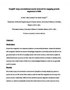
Figure 4: Processing flow of the change-based convolution algorithm. Custom processing kernels are shown in blue, processing steps using available libraries are shown in green, variables sharable among layers are shown in yellow, and variables to be stored per-layer are colored orange. The size and data type of the tensor storing the intermediate results is indicated below each the variable name.

No ground truth available Frame 1

Frame 2

full-frame change-based

...

Table 1: Performance Baseline Compute Time Breakdown

Ground Truth Frame 6

Layer

evaluation

Frame 5

1 2 3 4 5

Frame 6

change-based change-based

Figure 5: Scheme of the image sequence used for the evaluations.

them from the first to the last layer, sweeping the threshold parameter for each layer and keeping the maximum value before a clear performance degradation became noticeable when evaluating the entire validation set. The following evaluations will show that these thresholds need not be re-calibrated per video sequence and neither the accuracy nor the speed-up are overly sensitive to them.

4

RESULTS & DISCUSSION

In this section, we will first present the evaluation environment and analysis the baseline compute time breakdown. We then show how the threshold parameters have been selected before discussing throughput measurements and the accuracy-throughput trade-off. Finally, we discuss the compute time breakdown and how changes propagate through the network to confirm the quality of our GPU implementation and justify design choices made during the construction of the algorithm.

4.1

Evaluation Environment

While the algorithm is not limited to scene labeling/semantic segmentation, we perform our evaluations on the urban surveillance dataset described in [5] and using the corresponding scene labeling CNN, not using the multispectral imaging data. The dataset provides 51 training images and 6 validation images with 776 × 1040 pixel with the corresponding ground-truth scene labeling, classifying each pixel into one of the following 8 classes: building, road, tree, sky, tram, car/truck, water, distant background. For the validation set, the labeled images are part of short video sequences with 5 additional frames available before the frame for which the ground truth labeling is available. A trained network on this data is described in [5] and its parameters are reused unaltered for our evaluations. The procedure with which we perform our evaluation is visualized in Figure 5. We have implemented the proposed algorithm using CUDA and wrapped them as modules for the Torch framework [10]. We have evaluated the performance on a Jetson TX1 board with JetPack 2.3.1 (Nov. 2016). Our performance baseline for the entire CNN and for the change-based implementation the pixel-wise classification is relying on Nvidia’s cuDNN v5.1.5, which includes optimizations such

Conv.

Activ.

Pooling

total

share

72.9 ms 116.2 ms 302.8 ms 12.7 ms 1.6 ms

7.4 ms 6.9 ms 6.6 ms 1.7 ms —

3.3 ms 3.3 ms — — —

83.6 ms 126.4 ms 309.4 ms 14.4 ms 1.6 ms

15.6% 23.6% 57.8% 2.7% 0.3%

as the Winograd algorithm and FFT-based convolutions mentioned in Section 2.2.

4.2

Baseline Throughput and Computation Breakdown

Before we discuss the performance of the proposed algorithm, we analyze the baseline throughput and compute time breakdown in Table 1. Clearly, most time is spent performing convolutions, and the layers 1–3 performing 7 × 7 convolutions and belonging to the feature extraction part of the network are dominant with 91.9% (492 ms) of the overall computation time (535 ms or 1.87 frame/s). We thus specifically focus our analyses on these 3 layers, replacing only them with our CBconv layer.

4.3

Threshold Selection

Our algorithm introduces a threshold parameter for each layer, for which we outline the selection process in Section 3.3. While we might want to leave them variable to investigate a throughput against accuracy trade-off, we also want to ensure that not a single layer’s threshold is limiting the overall accuracy by aligning the tipping point where the accuracy starts to drop. We choose the thresholds conservatively, accepting very little accuracy drop, since any classification error will be focused around the moving objects which are our area of interest. We sweep the parameters of each layer to determine the increase in error (cf. Figure 6). We do so first for Layer 1 with τ2 = τ3 = 0 and select τ1 = 0.04, before repeating it for layers 2 and 3 after each other and using the already chosen thresholds for the previous layers, selecting τ2 = 0.3 and τ3 = 1.0. With this selection of thresholds we can scale them jointly to analyze the trade-off against the classification accuracy more concisely (cf. Figure 7, left). The accuracy of the individual test sequences are visualized, and clearly show a similar behavior with a plateau up to a clear point where there is a steep increase in error rate.

4.4

Throughput Evaluations

The motivation for the entire proposed algorithm was to increase throughput by focusing only on the frame-to-frame changes. We

Error Incr. [%]

arXiv preprint, v2, June 2017

L. Cavigelli et al.

0.8 0.6 0.4 0.2 0 0

0.1 5 · 10−2 Threshold for Layer 1 (τ1 )

0.15

0

0.2 0.4 0.6 0.8 1 Threshold for Layer 2 (τ2 )

0

1 2 3 Threshold for Layer 3 (τ3 )

0.4 0.2 0

Throughput [frame/s]

0.6

# Changed pixels

Classif. Error Increase [%]

Figure 6: Analysis of the increase in pixel classification error rate by selecting a certain change detect threshold. This analysis is conducted layer-by-layer, where the error increase of any layer includes the error introduced by the previous layers’ threshold choice (τ1 = 0.04, τ2 = 0.3, τ3 = 1.0).

106

105

104 0

0.5 1 1.5 Threshold Factor

2

0

0.5 1 1.5 Threshold Factor

2

25 20 15 10 5 0

cuDNN 0

0.5 1 1.5 Threshold Factor

2

show the performance gain in Figure 7 (right) with the indicated baseline analyzing the entire frame with the same network using cuDNN. In the extreme case of setting all thresholds to zero, the entire frame is updated, which results in a clear performance loss because of the change detection overhead as well as fewer optimization options such as less cache-friendly access patterns when generating the X matrix. When increasing the threshold factor, the throughput increases rapidly to about 16 frame/s, where it starts saturating because the change detection step as well as other non-varying components like the pooling and pixel classification layers are becoming dominant and the number of detected changed pixels does not further decrease. We almost reach this plateau already for a threshold factor of 1, where we have by construction almost no accuracy loss. The average frame rate over the different sequences is near 17 frame/s at this point—an improvement of 8.6× over the cuDNN baseline of 1.96 frame/s. One sequence ( ) has—while still being close to 5.1× faster than the baseline—a significantly lower throughput than the other sequences. While most of them show typical scenarios such as shown in Figure 3, this sequences shows a very busy situation where the entire road is full of vehicle and all of them are moving. The aggregate number of changed pixels across all 3 layers is visualized in Figure 7 (center). Most sequences trigger less than 3% of the maximum possible number of changes while the aforementioned exceptional case has a significantly higher share of around 9%. We have repeated the same evaluations on a workstation with a Nvidia GTX Titan X GPU, obtaining an almost identical throughputthreshold trade-off and compute time breakdown up to a scaling

Throughput [frame/s]

Figure 7: Evaluation of the impact of jointly scaling the change detection thresholds on the classification error, the number of detected changed pixels (sum over all 3 layers), and the throughput.

25 20 15 10 5 0

cuDNN 92

94 96 98 Pixel Classification Accuracy [%]

Figure 8: Evaluation of the throughput-accuracy trade-off for all 6 video sequences.

factor of 11.9×—as can be expected for a largely very well parallelizable workload and a 12× more powerful device with a similar architecture (TX1: 512 GFLOPS and 25.6 GB/s DRAM bandwidth, GTX Titan X: 6144 GFLOPS and 336 GB/s).

4.5

Accuracy-Throughput Trade-Off

While for some scenarios any drop in accuracy is unacceptable, many applications allow for some trade-off between accuracy and throughput—after all choosing a specific CNN already implies selecting a network with an associated accuracy and computational cost. We analyze the trade-off directly in Figure 8. The most extreme case is updating the entire frame every time resulting in the lowest

CBinfer: Change-Based Inference for Convolutional Neural Networks on Video Data

arXiv preprint, v2, June 2017

L1 Conv. L2 Conv. L3 Conv.

0

0.2

0.4

0.6

0.8

1

1.2

1.4

Compute Time [ µs ] Change Det.

Change Extr.

gen. X

1.6

1.8

b) Layer 2 worst-case

·104 GEMM

Output Upd.

Figure 9: Compute time for the individual processing steps per layer running on the GPU for a typical frame sequence. a) Layer 1 changes

throughput at the same accuracy as full-frame inference. Increasing the threshold factor in steps of 0.25 immediately results in a significant throughput gain and for most sequences the trade-off only starts at frame rates close to saturation above 16 frame/s. The same frame sequence already deviate from the norm before behaves differently here as well. However, an adaptive selection of the threshold factor such as a simple control loop getting feedback about the number of changed pixels could allow for a guaranteed throughput by reducing the accuracy in such cases and is left to be explored in future work.

4.6

Compute Time Breakdown

In Section 4.2 and specifically in Table 1, we already discussed the compute time breakdown of the entire network when using frameby-frame analysis. To gain more in-depth understanding of the limiting factors of our proposed algorithm, we show a detailed compute time breakdown of only the change-based convolution layers in Figure 9. The time spent on change detection is similar across all 3 conv layers, which aligns well with our expectations since the feature map volume at the input of nch · h · w values is identical for L2 and L3, and 25% smaller for L1. That this step already makes up for more than 23.4% of the overall time underlines the importance of a very simple change detection function: any increase in compute time for change detection has to be offset by time savings in the other steps by reducing the number of changes significantly. The change indexes extraction effort is linear to the number of pixels h · w and the clear drop from L1 to L2 is as expected. However, since it is not well parallelizable, there is not much additional gain when comparing L2 to L3. The effort to generate the X matrix is very dependent on the number of changed pixels, the number of feature maps, and the filter size. It is however mostly important that the time spent on shuffling data around to generate X is significantly smaller than the actual matrix multiplication, which clearly makes up the largest share. The subsequent update of the output values including activation only uses a negligible part of the overall processing time. An important aspect is not directly visible: The overall compute time for the critical part, the convolution and activation of L1-L3, has shrunk tremendously by more than 12.9× from 512.8 ms to about 39.7 ms. The remaining steps like polling (total 6.6 ms) and pixel-wise classification (L4, L5; total 16.0 ms) now take 36% of the compute time, such that they move more into the target of future optimizations.

c) Layer 2 changes

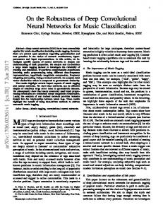
Figure 10: Analysis of the change propagation. (a) shows the changes detected in Layer 1 using the thresholds determined in Section 4.3, in the upper part of the image there are several single-pixel changes due to noise. We show the changed pixels for Layer 2 based on worst-case propagation as assumed when dropping the Layer 2 change detection step (b) and those when applying change detection instead (c).

4.7

Change Propagation

During the construction of the algorithm we argued that change detection should be performed for every convolution layer not only for modularity, but also justifying that the worst-case change propagation we had to assume otherwise would result in a higher computational effort. We have experimentally verified this and show an example case in Figure 10. For Layer 2, the number of changes is reduced by 6.8× from 7.57% to 1.11% and for Layer 3 from 2.58% to 1.94% by 1.33×. While it clearly pays of for Layer 2, we analyze the situation for Layer 3 more closely. From the previous section, we know that the change detection makes up for only 22% of the overall compute time in Layer 3 and scaling up the time to generate the X matrix, perform the matrix multiplication and update the output clearly exceeds the overhead introduced by the change detection step. The change extraction step cannot be dropped, and in fact the change detection has to be replaced with a (though very quick to evaluate) change propagation kernel.

4.8

Energy Efficiency

We have measured the current consumption of the entire Jetson TX1 board with only an Ethernet connection and no other off-board peripherals, running a continuous CNN workload. The average current when running the baseline cuDNN-based implementation was measured at 680 mA (12.9 W). The power consumption dropped to 10.92 W when running CBinfer. When idling, we measured 1.7 W under normal conditions, which raised to 2.5 W when enforcing the maximum clock frequency, as has been done to maximize throughput for the earlier measurements. The CNN we used has a computational complexity of 210 GOp/frame, where the number of operations (Ops) is the sum of additions and multiplications required for the convolution layers. We thus obtain 413 GOp/s and 32.0 GOp/s/W with the cuDNN baseline. With the proposed CBinfer procedure, we obtain a per-frame inference equivalent throughput of 3577 GOp/s and an energy efficiency boost of about 10× to 327.6 GOp/s/W.

arXiv preprint, v2, June 2017

5

CONCLUSION

We have proposed and evaluated a novel algorithm for changebased evaluation of CNNs for video recorded with a static camera setting, exploiting the spatio-temporal sparsity of pixel changes. The results clearly show that even when choosing the change detection parameters conservatively to introduce no significant increase in misclassified pixels during semantic segmentation, an average speed-up of 8.6× over a cuDNN baseline has been achieved using an optimized GPU implementation. An in-depth evaluation of the throughput-accuracy trade-off shows the aforementioned performance jump without loss and shows how the throughput can be further increased at the expense of accuracy. Analysis of the compute time split-up of the individual steps of the algorithm show that despite some overhead the GPU is fully loaded performing multiply-accumulate operations to update the changed pixels using the highly optimized cuBLAS matrix multiplication. An analysis of how changes propagate through the CNN further underline the optimality of the structure of the proposed algorithm. The resulting boost in energy efficiency over per-frame evaluation is an average of 10×, equivalent to 328 GOp/s/W on the Tegra X1 platform.

ACKNOWLEDGMENTS The authors would like to thank armasuisse Science & Technology for funding this research. This project was supported in part by the EU’s H2020 programme under grant no. 732631 (OPRECOMP).

REFERENCES [1] Sami Abu-El-Haija, Nisarg Kothari, and others. 2016. YouTube-8M: A Large-Scale Video Classification Benchmark. (2016). [2] Alessandro Aimar, Hesham Mostafa, and others. 2017. NullHop: A Flexible Convolutional Neural Network Accelerator Based on Sparse Representations of Feature Maps. IEEE Transactions on Very Large Scale Integration Systems (2017). [3] Renzo Andri, Lukas Cavigelli, and others. 2016. YodaNN: An Ultra-Low Power Convolutional Neural Network Accelerator Based on Binary Weights. In Proc. IEEE ISVLSI. 236–241. [4] Lukas Cavigelli and Luca Benini. 2016. Origami: A 803 GOp/s/W Convolutional Network Accelerator. IEEE TCSVT (2016). [5] Lukas Cavigelli, Dominic Bernath, and others. 2016. Computationally efficient target classification in multispectral image data with Deep Neural Networks. In Proc. SPIE Security + Defence, Vol. 9997. [6] Lukas Cavigelli, David Gschwend, and others. 2015. Origami: A Convolutional Network Accelerator. In Proc. ACM GLSVLSI. ACM Press, 199–204. [7] Lukas Cavigelli, Michele Magno, and Luca Benini. 2015. Accelerating Real-Time Embedded Scene Labeling with Convolutional Networks. In Proc. ACM/IEEE DAC. [8] Yu-Hsin Chen, Tushar Krishna, and others. 2016. Eyeriss: An energy-efficient reconfigurable accelerator for deep convolutional neural networks. In Proc. IEEE ISSCC. 262–263. [9] Sharan Chetlur, Cliff Woolley, and others. 2014. cuDNN: Efficient Primitives for Deep Learning. [10] Ronan Collobert. 2011. Torch7: A Matlab-like Environment for Machine Learning. Advances in Neural Information Processing Systems Workshops (2011). [11] Marius Cordts, Mohamed Omran, and others. 2016. The Cityscapes Dataset for Semantic Urban Scene Understanding. In Proc. IEEE CVPR. 3213–3223. [12] Matthieu Courbariaux, Yoshua Bengio, and Jean-Pierre David. 2015. BinaryConnect: Training Deep Neural Networks with binary weights during propagations. In Adv. NIPS. 3105–3113. [13] Jia Deng, Wei Dong, and others. 2009. ImageNet: A large-scale hierarchical image database. In Proc. IEEE CVPR. [14] Clement Farabet, Berin Martini, and others. 2011. NeuFlow: A Runtime Reconfigurable Dataflow Processor for Vision. In Proc. IEEE CVPRW. 109–116. [15] Nicolas Farrugia, Franck Mamalet, and others. 2009. Fast and Robust Face Detection on a Parallel Optimized Architecture Implemented on FPGA. IEEE TCSVT 19, 4 (2009), 597–602. [16] Philipp Fischer, Alexey Dosovitskiy, and others. 2015. FlowNet: Learning Optical Flow with Convolutional Networks. In arXiv:15047.06852.

L. Cavigelli et al. [17] Philipp Gysel, Mohammad Motamedi, and Soheil Ghiasi. 2016. Hardwareoriented Approximation of Convolutional Neural Networks. In ICLR Workshops. [18] Song Han, Xingyu Liu, and others. 2016. EIE: Efficient Inference Engine on Compressed Deep Neural Network. arXiv:1602.01528 (2016). [19] Soheil Hashemi, Nicholas Anthony, and others. 2016. Understanding the Impact of Precision Quantization on the Accuracy and Energy of Neural Networks. arXiv:1612.03940 (2016). [20] Kaiming He, Xiangyu Zhang, and others. 2015. Deep Residual Learning for Image Recognition. Proc. IEEE CVPR (2015), 770–778. [21] Kaiming He, Xiangyu Zhang, and others. 2015. Delving Deep into Rectifiers: Surpassing Human-Level Performance on ImageNet Classification. [22] David Held, Sebastian Thrun, and Silvio Savarese. 2016. Learning to track at 100 FPS with deep regression networks. LNCS 9905 (2016), 749–765. [23] Forrest N. Iandola, Matthew W. Moskewicz, and others. 2016. SqueezeNet: AlexNet-Level Accuracy with 50x Fewer Parameters and 1MB Model Size. arXiv:1602.07360 (2016). [24] Max Jaderberg, Andrea Vedaldi, and A Zisserman. 2014. Speeding up Convolutional Neural Networks with Low Rank Expansions. In arXiv:1405.3866. [25] Yangqing Jia. 2013. Caffe: An Open Source Convolutional Architecture for Fast Feature Embedding. (2013). http://caffe.berkeleyvision.org [26] Jonghoon Jin, Vinayak Gokhale, and others. 2014. An efficient implementation of deep convolutional neural networks on a mobile coprocessor. In Proc. IEEE MWSCAS’14. 133–136. [27] Andrej Karpathy, George Toderici, and others. 2014. Large-scale video classification with convolutional neural networks. Proc. IEEE CVPR (2014), 1725–1732. [28] Alex Krizhevsky, Ilya Sutskever, and Geoffrey E Hinton. 2012. Imagenet Classification With Deep Convolutional Neural Networks. In Adv. NIPS. [29] Herman Kruegle. 1995. CCTV Surveillance: Video Practices and Technology. Butterworth-Heinemann, Woburn, MA, USA. [30] Andrew Lavin. 2015. maxDNN: An Efficient Convolution Kernel for Deep Learning with Maxwell GPUs. In arXiv:1501.06633v3. [31] Andrew Lavin and Scott Gray. 2016. Fast Algorithms for Convolutional Neural Networks. In Proc. IEEE CVPR. 4013–4021. [32] Hao Li, Asim Kadav, and others. 2016. Pruning Filters for Efficient ConvNets. arXiv:1608.08710 (2016). [33] Tsung-Yi Lin, Michael Maire, and others. 2014. Microsoft COCO: Common Objects in Context. In Proc. ECCV. [34] Jonathan Long, Evan Shelhamer, and Trevor Darrell. 2015. Fully Convolutional Networks for Semantic Segmentation. In Proc. IEEE CVPR. [35] Woon-sung Park and Munchurl Kim. 2016. CNN-based in-loop filtering for coding efficiency improvement. In Proc. IEEE Image, Video, and Multidimensional Signal Processing Workshop. [36] Adam Paszke, Abhishek Chaurasia, and others. 2016. ENet: A Deep Neural Network Architecture for Real-Time Semantic Segmentation. In arXiv:1609.02147. [37] Fatih Porikli, Francois Bremond, and others. 2013. Video surveillance: past, present, and now the future [DSP Forum]. IEEE Signal Processing Magazine 30 (2013), 190–198. [38] Mohammad Rastegari, Vicente Ordonez, and others. 2016. XNOR-Net: ImageNet Classification Using Binary Convolutional Neural Networks. In arXiv:1603.05279. [39] Joseph Redmon, Santosh Divvala, and others. 2016. You Only Look Once: Unified, Real-Time Object Detection. [40] Shaoqing Ren, Kaiming He, and others. 2015. Faster R-CNN: Towards Real-Time Object Detection with Region Proposal Networks. arXiv:1506.01497 (2015). [41] Olga Russakovsky, Jia Deng, and others. 2015. ImageNet Large Scale Visual Recognition Challenge. IJCV 115, 3 (2015), 211–252. [42] Evan Shelhamer, Kate Rakelly, and others. 2016. Clockwork Convnets for Video Semantic Segmentation. arXiv:1608.03609 (2016). [43] Christian Szegedy, Wei Liu, and others. 2015. Going Deeper with Convolutions. In Proc. IEEE CVPR. [44] Nicolas Vasilache, Jeff Johnson, and others. 2014. Fast Convolutional Nets With fbfft: A GPU Performance Evaluation. arXiv:1412.7580 (2014). [45] Chen Zhang, Zhenman Fang, and others. 2016. Caffeine: Towards Uniformed Representation and Acceleration for Deep Convolutional Neural Networks. In Proc. ACM ICCAD. New York, NY, USA. [46] Kaihua Zhang, Qingshan Liu, and others. 2016. Robust Visual Tracking via Convolutional Networks without Training. IEEE TIP (2016). [47] Qian Zhang, Ting Wang, and others. 2015. ApproxANN: An Approximate Computing Framework for Artificial Neural Network. In Proc. IEEE DATE.