Ceiling Light Landmarks Based Localization and Motion ... - FUSION

Proceedings of the 2007 IEEE International Conference on Networking, Sensing and Control, London, UK, 15-17 April 2007

MonA01

Ceiling Light Landmarks Based Localization and Motion Control for a Mobile Robot Hongbo Wang, Hongnian Yu and Lingfu Kong

Abstract—This paper presents ceiling light landmarks based localization and motion control for a mobile robot. The novel mechanism design for the mobile robot is introduced, and the method of localization using ceiling light is proposed. Navigation map, network matrix and the method to find shortest path are described. From the path planning, the control scheme of autonomous navigation for the mobile robot can be generated automatically. Navigational experiments indicate the effectiveness of the method presented in the paper.

T

II. MECHANICAL DESIGN

I. INTRODUCTION

o navigate effectively in a fairly complex workspace, an intelligent autonomous mobile robot system needs to be able to determine the state of its world and its own location with respect to its immediate surroundings. Such self-location is critical for the reliable performance of an autonomous system. Many methods are used to provide self-location in mobile robots. These methods can be roughly categorized as relative position measurements and absolute position measurements [1]. Among the above methods, landmarks probably provide the best information for mobile robots localization. Several researchers have approached the problem of self-location in mobile robots by employing landmarks [2]-[4]. The key idea of self-location is to use special marks that include a wealth of geometric information under perspective projection so that the camera location can be easily computed from the image of the guide marks. Researchers have chosen ceiling lights as landmarks since they can be easily detected due to the high contrast between the light and the ceiling surface. Also, the ceiling lights do not require to be specially installed [5], [6]. Therefore, we choose ceiling lights as landmarks to realize the mobile robot localization. With this positing function, the mobile robot developed here is capable of moving along any path in an environment where ceiling lights have been installed. A major problem in reaching the goal of mobile robot is the path planning or find-path problem. This problem can be stated as: given an initial position, a goal, possible paths and a set of obstacles distributed in space, find a continuous and shortest path without colliding with any obstacle along the

Manuscript received November 7, 2006. Hongbo Wang is with Robotics Institute, Yanshan University, 066004, Qinhuangdao, P. R. China ([email protected]). Hongnian Yu is with the Faculty of Computing, engineering and technology, Staffordshire University, Stafford, ST18 0DG, UK ([email protected]). Lingfu Kong is with School of Information Technology and Engineering, Yanshan University, 066004, Qinhuangdao, Hebei Province, P. R. China ([email protected]).

1-4244-1076-2/07/$25.00 ©2007 IEEE

path. Many path planning algorithms on mobile robots have been proposed [7]-[9]. Our path planning is based on the navigation map composed of landmarks. This paper describes mechanical design, localization and path planning for a mobile robot. Based on the path planning, the motion control for autonomous navigation of the mobile robot is proposed. Finally, an example of path planning and navigational experiment are given.

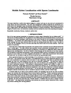
The mechanism of a mobile robot with 8 wheels is shown in Fig.1 and Fig.2. The 8 wheels are divided into 4 groups that have same transmission system. The one wheel of each group is driving wheel and another is free wheel. The transmission system has two degrees of freedom. Two belts driven by two motors make the 4 driving wheels move in synchronous way. As shown in Fig.2, the one of two belts is navigational driving belt and another is rotational driving belt.

Fig. 1 A omni-directional mobile robot

Fig. 2 Driving system of mobile robot

The mobile robot is an omni-directional mobile robot that can change the navigating direction with any rotation radium. However, the mobile robot cannot change the orientation of the platform. The motion of the platform is a plane translation. Therefore, for the localization and navigation control, we only need to recognize the position of the mobile robot.

285

III. POSITING ALGORITHM To enable the mobile robot locate and navigate itself, we have chosen ceiling lights as landmarks. In this paper, the double ceiling lights are used. For the double lights, a three-dimensional image processing method is proposed to determine the coordinate system of the ceiling light. From the raster coordinates of the double lights, we have the vectors p i = ( xui y ui f ) (i=1, 2, 3, 4) in the camera coordinate system shown in Fig. 3. The position vectors q i (i=1, 2, 3, 4) of the light ends relative to camera coordinate system can be determined using the following image processing method. From perspective transformation, the relation between q i and p i can be expressed as

q i = k i p i (i=1, 2...4),

Using a similar method, the proportionality coefficients k 2 and k 4 can be expressed as follows

p 2 ⋅ (p 3 × p1 ) , (6) p 2 ⋅ (p 3 × p 4 ) p ⋅ (p × p ) k 2 = c21k1 , c21 = 3 4 1 . (7) p 3 ⋅ (p 4 × p 2 ) Since the distance between Q1 and Q2 is the length of the k 4 = c41k1 , c41 =

light, the following equation can be obtained 2 2 k 2p 2 − k1p1 = k1 p12 − 2c21 (p1 ⋅ p 2 ) + c21 p2 .

From the above equation, the proportionality coefficient k1 can be calculated

(1)

yj

zj oi

Q2

xj

Q1

q 2 = k 2p 2

qcj

q 1 = k1 p1

xc

p2 p3

P4

Ceiling Plane

systems of the light and the camera can be established. The light coordinate system o − xyz is set as shown in Fig. 3. The origin o of the light coordinate system is chosen at the

q 4 = k 4p 4

midpoint of points Q1 and Q3 . The position vector of the

P1

origin is q c = (q 3 + q1 ) / 2 . The x -axis is along the

Image Plane

direction from Q2 to Q1 . The z -axis is along the normal line of the plane that is composed of three points Q1 , Q2 ,

oc

yc Fig. 3 Relation between the coordinate systems of the camera and the double lights

and Q3 . The unit vector of z -axis can be determined as

camera coordinate system, and ki is the proportionality coefficient between two vectors. Since the two lights are parallel and the lengths of the two lights are equal, the following vector equation can be obtained k1p1 − k 2p 2 = k 4p 4 − k3p 3 . (2) Using the p 4 cross product with the above equation, we have the following equation k1 (p 4 × p1 ) − k 2 (p 4 × p 2 ) = − k 3 (p 4 × p 3 ) . (3) Using the p 2 inner product with the above equation, the following equation can be obtained k1p 2 ⋅ (p 4 × p1 ) = − k3p 2 ⋅ (p 4 × p 3 ) . (4) The ratio of k3 to k1 can be expressed in the following

k3 = c31k1 , c31 = −

(9)

After q i is obtained, the relation between the coordinate

p1 p4

equation

.

equations (5), (6), and (7). From the equation (1), the q i (i=1, 2, 3, 4) can be calculated.

zc P2 P 3

2 2 p12 − 2c21 (p1 ⋅ p 2 ) + c21 p2

Once k1 is known, the k 2 , k3 and k 4 can be obtained using

Q4

Q3 q 3 = k3p 3

q 2 − q1

k1 =

where q i indicates the position vector of light end Qi in the Ceiling Light

(8)

p 2 ⋅ (p 4 × p1 ) . p 2 ⋅ (p 4 × p 3 )

(5)

follows

(q 4 − q 3 )× (q1 − q3 ) . (q 4 − q 3 )× (q1 − q3 )

ez =

(10)

The unit vector of the y -axis can be determined using right hand rule. The transformation matrix of the light coordinate system relative to camera coordinate system can be expressed as follows A = ex e y ez , (11)

[

]

The position of the mobile robot in the light coordinate system can be determined as follows

q jc = − A T q cj .

(12)

When only one landmark is in sight of the camera, we assume the landmark is j-th ceiling light. Since the position vector of the j-th ceiling light in the world coordinate system is known, the position vector of the mobile robot in a two-dimensional world coordinate system o − xy can be obtained as follows

286

roc = roj + r jc ,

B. Shortest Path Algorithm

(13)

where r is a two-dimensional vector with x and y coordinates. IV. PATH PLANNING A. Navigation Map and Network Matrix Navigation of a mobile robot using landmarks depends upon a navigation map shown in Fig. 4. The navigation map should contain information about the position of every landmark and about possible paths. The possible paths are determined as a series of lines that connect neighboring nodes situated near the landmarks. The navigation map with n landmarks can be expressed using the following matrices:

Nodek d jk

rk y

1

" r0i "

rj x

o

ri

Node j

2

3

i

d ijm .

D N is the matrix of shortest path length whose i, j-th element expresses the length of the shortest path among all nodes.

pijl indicates the next-to-last node in the shortest path

(14) (15)

landmarks (ceiling lights) in the world coordinate system. Matrix ∆R indicates the position vector of every node relative to the corresponding landmarks. This matrix determines the navigational course drift from the landmarks taking into consideration the obstacles in the path. The position vectors of all nodes can be expressed as R node = r1 r2 " rn = R mark + ∆R . (16)

]

In order to find the optimal path among all possible paths, we introduce the following network matrix

0  0 d D 0 =  21 "  0  d n1

d120 0 " d n02

0

m

From this definition of d ij , it follows that d ij denotes the

D m denotes the m × m matrix whose i, j-th element is

Matrix R mark is composed of the position vectors of all

[

m

intermediate node. If no such path exists, then let d ij = ∞ .

∆rii

Fig. 4. Navigation map

∆R = [∆r11 ∆r22 " ∆rnn ] .

node j, where only the first m-1 node is allowed to be the

d ijN represents the length of a shortest path form i to j.

Landmark

R mark = [ro1 ro 2 " ron ] ,

d ijm denotes the length of a shortest path from node i to

length of the shortest path from i to j that uses no intermediate nodes.

n

"

0

Based on the network matrix D , the shortest path from the starting position to the selected node (goal position) can be found where we only specify a starting and a goal position. Here, the “Floyd Shortest Path Algorithm” is used to find the shortest path [10]. Before introducing the algorithms, some notations need to be defined:

from i to j that is called the penultimate node of that path. s represents the path vector of the shortest path whose every element is the node number (landmark number). Suppose the shortest path consists of L nodes, then

pijl (l = 1,2,3,...L)

constitutes

the

path

vector

s = (s1 , s2 " sL ) of the shortest path, where sl = pijL −l +1 . 0

The “Floyd Shortest Path Algorithm” starts with D and 1

0

2

1

calculates D from D . Next, D is calculated from D . N −1

N

This process is repeated until D is obtained from D . The algorithm can be described as follows: Step 1: From the navigation map, determine the network 0

matrix D . Step 2: For m=1,2, … N, successively determine the elements

" d10n   " d 20n  , " "  " 0 

m

of D from the elements of D recursive formula

(17)

{

m −1

using the following

}

m −1 d ijm = min d imm −1 + d mj , d ijm −1 .

0

where d ij indicates the distance between node i and j, that is,

d ij0 = ri − r j . If there is an obstacle between node i and j, or 0

node i and j are not adjacent, we use d ij = ∞ to express that the path between node i and j is not feasible. Since the distance from node i to j and the distance from node j to i are equal, the network matrix is a symmetry matrix.

(18)

As each element is determined, it records the path it represents. Upon termination, the i, j-th element of matrix

D N represents the length of a shortest path from node i to j. m Note that d ii = 0 for all i and all m. Hence, the diagonal 1

2

N

elements of the matrices D , D , ... D do not need to be m −1

m

m −1

m

calculated. Since d im = d im and d mi = d mi for all i=1,2, m

… N, in the computation of matrix D , the m-th row and 0

m-th column need not be calculated. Moreover, D is a

287

m

symmetry matrix. Hence, only d ij (j>i) is calculated in m

matrix D . Step 3: After D

N

l

is obtained, the penultimate node pij can L

1

N

0

be found as follows: Let pij = j and pij = i . If pij = pij , there are only two nodes in the shortest path and the path L

1

vector from i to j is s = (i, j ) = ( pij , pij ) . Otherwise, for

pijl (l = 1,2,3,...L − 1) , suppose that the penultimate node in a shortest path from i to j is any node k , that is,

pijl = k (k ≠ i, j and is not repeated). If k is satisfied with the following equation

d ikN + d kj0 = d ijN ,

(19)

2

we have pij = k . Then, the second-to-last node in this path 3

is the penultimate node pik on a shortest path from i to k. This process can be repeated until all the nodes in this path 0

from i to j have been tracked back. In this step, only D and

D N matrices are required for the value of k to be

 (a i +1 × a i ) ⋅ k   , a ⋅ a i +1 i  

α = tan −1 

where k represents the normal unit vector of the plane o-xy. Using the above equation, we can obtain the control scheme for the mobile robot from node i+1 to node i+2. When α < 0, the mobile robot turns α degree to the right, otherwise, it turns α degree to the left. In the above control scheme, the mobile robot must navigate along the vector a i and the moving direction must be coincident with the direction of the vector a i . However, when a mobile robot navigates itself from node i to node i+1, it will unavoidable encounter an obstacle. After the obstacle is avoided, the mobile robot will drift off the vector a i as shown in Fig. 6. In order to enable the mobile robot to move to node i+1 after obstacle avoidance, the moving direction of the mobile robot should be calculated. From the feature of our mobile robot, when the output angle of rotation driving wheel is fixed, the mobile robot moves along a straight line. The moving direction of the mobile robot can be obtained as follows:

determined. Step 4: When all the nodes in the shortest path from i to j have been found, the path vector from i to j can be obtained as follows

(

)

s = (s1 , s 2 " s L ) = pijL , pijL −1 " p1ij .

y Nodei +1 ai

(20) Nodei

V. MOTION CONTROL BASED ON PATH PLANNING

y

Nodei +1 Node i •

•

ai

α

θ

•

In this section, we will present the control scheme for the autonomous navigation of the mobile robot based on the path vector. When the path vector is known, the position vectors of all nodes in the shortest path can be expressed in the following matrix

rsi

γ a i +1

β

di

Position of Robot

rom

Nodei+ 2 •

ci Moving Direct ion of Robot

x

o

Fig. 6 Position and moving direction of robot after obstacle avoidance 0

0

n −1

n −1

(1) Take n pairs of coordinates ( romx , romy ) , … ( romx , romy ) from present position to the position before n-1 control cycles as shown in Fig. 7. y

ai +1

n −1

n −1

( romx , romy ) 1 1 ( romx , romy )

Nodei + 2

n −1 rom

rsi + 2

0 0 ( romx , romy )

1 rom

ci rom

x

o

• bi

• rsi +1

(23)

Moving Direct ion of Robot

Fig. 5 Vectors between adjoining nodes

R s = [rs1

rs 2 " rsm ] .

o

(21)

x

Fig. 7 Determination of moving direction for mobile robot

From Fig. 5, two vectors adjoining three nodes in the path can be expressed as a i = rsi +1 − rsi , a i +1 = rsi + 2 − rsi +1 (i L , the mobile robot has not yet reached the node i+1. When | a i |≤ L has been obtained, node i+1 has been

1800 3600 5900 7200  0  1800 0 1800 4100 5400   3600 1800 0 2300 3600  5900 4100 2300 0 1300   7200 5400 3600 1300 0   9000 7200 5400 3100 1800  2900 4700 6500 8800 10100   4700 6500 4700 7000 8300  6500 4700 2900 5200 6500   9078 7278 5478 3178 2900  10613 8813 7013 4713 3413  5800 7600 8113 10413 11713   6313 8113 7600 9900 11200 11978 10178 8378 6078 5800  13778 11978 10178 7878 7600

arrived. In this case, the mobile robot can automatically turn to the right or to the left at angle γ and navigate from node i+1 to i+2.

Once the matrices D and D are known, the shortest path from node i to j can be found as a path

vector a i can be calculated as follows

L =| d i | cos θ + | b i | cos(γ − α ) .

(31)

When the distance between two nodes is bigger than the projection of the vectors b i and c i on vector a i , that is,

9000

2900

4700

6500

9078

10613

5800

7200

4700

6500

4700

7278

8813

7600

5400 3100

6500 8800

4700 7000

2900 5200

5478 3178

7013 4713

8113 10413

1800 0

10100 8300 11900 10100

6500 8300

2900 3413

3413 2900

11713 13513

11900

0

1800

3600

11978 13513

2900

10100 8300

1800 3600

0 1800

1800 0

10178 11713 8378 9913

3413 5213

3413 2900

11978 10178 13513 11713

8378 9913

0 1800

13513

2900

5213

13591 15126

3413

1800 0

13591 15126 0

13000 3413 2900 4700 10378 14613 1800 6313 14878 13078 11278 2900 4700 16491 8113

16678 14878 13078

0

4700

6500

18291

6313 11978 13778 10178 11978 8378 10178  6078 7878  11200 5800 7600   13000 6313 8113  3413 14878 16678  2900 13078 14878 4700 11278 13078  10378 2900 4700   14613 4700 6500  1800 16491 18291  0 15978 17778 15978 0 1800   17778 1800 0  8113

7600 9900

15

T

VI. EXAMPLE AND E XPERIMENTS Fig. 8 shows a visual navigation map in our experimental

vector s = (13 8 9 3 4 10 14) . The distance (15978 mm) of the shortest path can be obtained from the 15

element of 13-th row and 14-th column in matrix D .

289

We tested the navigation of the mobile robot along this navigation path. The mobile robot was able to navigate with a maximum position error of 100mm at the goal node as shown in Fig. 9.

Computational Intelligence in Robotics and Automation, Kobe, Japan, 2003, Vol. 2, pp. 1028-1033. [10] E. Minieka, “Optimization algorithms for networks and graphs,” Marcel Dekker, Inc. New York and Basel, 1978.

Position error along y-axis (mm)

120 80 40 0 -40 -80 -120 -120

-80

-40

0

40

80

120

Positin error along x-axis (mm)

Fig. 9 Position error of navigation experiments

VII. CONCLUSION This paper presents ceiling light landmarks based localization and motion control for a mobile robot. A novel mechanism of the mobile robot is introduced and the mobile robot localization is described. The navigation map that contains information about the position of every landmark and possible path in the navigational environment is established and the network matrix that expresses the navigation map is obtained. “Floyd Shortest Path Algorithm” is used to find the shortest path from among all possible paths while only a starting position and a goal position are given. From the shortest path vector, the motion control scheme to guide the mobile robot can be generated automatically. An example of path planning and navigational experiment indicate that the method presented in this paper is practical. REFERENCES [1] [2] [3] [4]

[5] [6] [7]

[8] [9]

J. Borenstein, H. R. Everett, L. Feng, and D. Wahe, “Mobile robot positioning: sensors and techniques,” J. Robotic Systems, 14(4), pp. 231-249, 1997. S. Se, D. Lowe, and J. Little, “Mobile robot localization and mapping with uncertainty using scale-invariant visual landmark,” International Journal of Robot Research, 21(8), pp.735-758, 2002. J. M. Armingol, A. de la Escalera, L. Moreno, and M. A. Salichs, “Mobile robot localization using a non-linear evolutionary filter,” Journal of Advanced Robotics, 16(7), 629-652, 2002. A. Bais, and R. Sablatnig, “Landmark based global self-localization of mobile soccer robots,” in Proceedings of the 7th Asian Conference on Computer Vision. Hyderabad, India, Springer Lecture Notes in Computer Science 3852, 2006, Vol.2, 842-85. H. S. Dulimarta, and A. K. Jain, “Mobile robot localization in indoor environment,” Pattern Recognition, 30(1), pp. 99-111, 1997. H. B. Wang and T. Ishimatsu, “Vision-based navigation for an electric wheelchair using ceiling light landmark,” Journal of Intelligent and Robotic Systems, Vol. 41, pp. 283-314, 2004. Y. Fukazawa, C. Trevai, J. Ota, H. Yuasa, T. Arai and H. Asama, “Region exploration path planning for a mobile robot expressing working environment by grid points,” in Proc. 2003 IEEE Int. Conf. Robotics and Automat., Taipei, Taiwan, 2003, pp. 2448-2454. J. P. Tu and S. X. Yang, “Genetic algorithm based Path Planning for a mobile robot,” ICRA 2003: pp. 1221-1226. A. M. Zhu and S. X. Yang, “Path Planning of multi-robot systems with cooperation,” in Proc. 2003 IEEE International Symposium on

290