Mobile Robot Localization using Ceiling Landmarks and Images. Captured from an RGB-D Camera. Wen-Tsai Huang, Chun-Lung Tsai and Huei-Yung Lin.
The 2012 IEEE/ASME International Conference on Advanced Intelligent Mechatronics July 11-14, 2012, Kaohsiung, Taiwan
Mobile Robot Localization using Ceiling Landmarks and Images Captured from an RGB-D Camera Wen-Tsai Huang, Chun-Lung Tsai and Huei-Yung Lin Abstract— In this work we propose two techniques for mobile robot localization for the indoor environment. First, we use the images of the markers attached on the ceiling with known positions to calculate the location and orientation of the robot, like a global method. Second, an RGB-D camera mounted on the robot is adopted to acquire the color and depth images of the environment, like a local method. The relative robot motion is then computed based on the registration of 3D point clouds and SURF features between the consecutive image frames. Since the uncorrelated sensing information is used by the above techniques, we have combined these two approaches to increase the robustness and accuracy of the localization. Experimental results and performance analysis are presented using real world image sequences.
I. INTRODUCTION In the robotics research areas, autonomous mobile localization has been studied by many researchers. The ability of autonomous localization generally means that a mobile robot is capable of recognizing the path and constructing a map under an unknown environment i.e. SLAM (Simultaneous Localization and Mapping). To know where the robot is, various kinds of sensors usually have to be used to acquire the external features from the environment, something like the senses of vision, touch, and hearing used by human to acquaint the external environment [12]. To acquire a robot’s position, there are mainly two kinds of approaches. One is to predict the displacement or position by a framework using probability theory. The other one is to apply a method based on three-dimensional reconstruction, making data registration for the information obtained from different viewpoints of the same object, and calculating the associated translation and orientation. The most commonly used and well-known technique of the former approach is the Kalman Filter [1], [2], which is a method based on estimation theory. It can be used to estimate the possible locations with the data obtained from the sensors with noisy measurement. In the previous work Negenborn described in detail about how to apply Kalman Filter for mobile robot localization [4]. The most common method for the latter approach is the ICP (Iterative Closest Point) algorithm proposed by Zhang [3]. It approximates the relative pose between two sets of data with iteration (pairwise registration) to obtain their translation and orientation. Usually the data come from laser rangers, sonars or depth cameras. This method is conceptually easy, but with The support of this work is in part by the National Science Council of Taiwan under Grant NSC-98-2221-E-194-041. The authors are with Department of Electrical Engineering and Advanced Institute of Manufacturing with High-tech Innovations (AIM-HI), National Chung Cheng University, 168 University Rd., Min-Hsiung, Chiayi 621, Taiwan, R.O.C.
978-1-4673-2576-9/12/$31.00 ©2012 IEEE
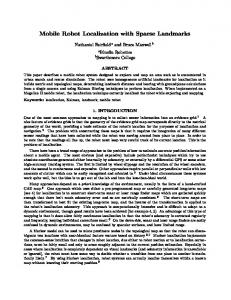
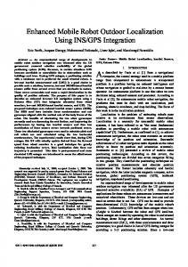
the drawbacks of slow in speed and insufficient accuracy in the results. In the paper, two techniques are proposed for mobile robot localization, namely a visual localization system based on the detection of pre-installed marker on the ceiling, and a vision system using the color and depth images captured from an RGB-D camera. Both techniques use the real-time detected image features to calculate the robot’s position, and no need for prior feature acquisition from any object in the environment, as well as training, etc. Furthermore, both approaches employ a camera as the primary sensor, i.e. just like human do with the eyes. For the RGB-D camera, it is also equipped with a depth sensor, which uses infrared to detect the distance between the scene and the camera. Although its precision is generally lower than the laser rangers, it is possible to integrate the information from color images to improve the acquisition results. II. LOCALIZATION WITH CEILING LANDMARKS In this technique, a simple concept based on triangulation is employed. Some specifically designed markers are installed on the ceiling in the indoor environment, and a camera is mounted on the robot and facing upward to capture their images. Just like sailors use the stars in the sky to localize themselves, the known positions of the markers are used to derive the robot’s location. This approach is similar to global localization. A. Marker Used in our System Fig. 1 shows the pattern of the markers used in our localization system. It is a black square pattern containing a few different combinations of white solid circles. The marker is designed to provide the unique localization information. This is achieved by assigning 3 out 4 corners as white solid circles. When the marker image is captured by a camera, it can be immediately identified without the influence of the camera’s viewpoint. Furthermore, the positions of the corner circles can be used to rectified the image and calculate the rotation information of the robot. As for the other circles in the pattern, they are used to indicate and distinguish the locations of the markers in the environment. B. Marker Detection The flow chart for marker detection is as shown in Fig. 2. Since the acquired images are color images and the markers are designed as black and white patterns, they are converted to grayscale images and then binarized for further processing. In this step the color information is also filtered to avoid false
855
Fig. 1 The marker pattern used in our system.
detection. Sobel edge detection algorithm is adopted to extract the makers from the white ceiling on the background.
can interest at four groups of points corresponding to the four corners of a square pattern. These four groups of points can be used to approximate the real corner locations by taking their average. After the corner location estimates are obtained by the point intersections, we employ Chen’s method [9] to move the detected corner points to sub-pixel precision positions according to the gradient information around the points as shown in Fig. 4. After the precise coordinates of the four corners are obtained, the center point coordinates of the marker can be calculated, as shown in Fig. 3(b). The amount of rotation can then be found according to pattern specification of four white circle positions. The other white circle positions in the pattern can thus be found, and the represented values of the marker patterns can be calculated. Since the points are assigned with known locations in the real environment, their coordinates can either be obtained or used as the origin to create a new coordinate system.
Fig. 2 The flowchart for marker detection.
After the edge detection is carried, there usually still exists some noise in the image; even the ceiling is almost white in the experiments. Thus, we apply morphological erosion and connected component labeling to filter out some small regions. With this process, the size of the noise region is usually getting smaller and smaller, and it is easy to identify the large components as potential marker patterns. In the previous step, the candidate labeling components are obtained. Whether those regions are really marker patterns need further investigation. We segment the image using the derived binary image, and the detected marker patterns are shown in Fig. 3(a) with blue bounding boxes. Consequently, line detection (Hough transform) can be used to detect the edges of the marker patterns.
(a)
(b)
Fig. 3 (a). The candidate label component is shown in blue bounding box. (b). The marker pattern is labeled with green lines, and the center point is indicated by a red dot.
Owing to the square feature of the constructed marker pattern, there should be four lines and four intersection points found in each pattern, and the angles between lines must be either 0◦ or 90◦ . Thus, the incorrect component can be easily filtered out of the detected line and corner features are not very complied. Due to the limitation of image resolution, it is possible that Hough transform results in multiple straight lines in very close locations. But even so, multiple near-by of Hough lines
Fig. 4 Move the angle points to sub-pixel precision. Assume that point q is in an angle point position close to the most precise subpixel position. (a). If p is in foreground region, the gradient of p will be zero. (b). If p is right on the edge, then the inner product of gradient p and vector qp should be equal to zero.
In the system setup, the camera is mounted on top of the robot and facing upward. If the tilt of the camera is not too severe, then the center point of the image coordinate system will be the image center, and it can be used to represent the relative position of the robot. That is, Ix and Iy in Eqs. (3) and (4) represent the x and y coordinates of the image center, and the detected marker pattern can use their center point as relative coordinates to the marker pattern, as Px and Py in Eqs.(3) and (4). If the distance between the camera and the ceiling is known, then these relative positions can be used to calculate the real position. In Eq. (1), h represents the distance between the camera and the ceiling, f is the focal length of the camera, l is the length of the marker pattern in the image. If this length l is unknown, then the physical dimension of the marker pattern can be used. For the rotation estimation, we only need to calculate the amount of rotation between two adjacent images detected with the same marker. The displacement can then be calculated by using the calculated rotation and the relative positions in the image coordinates. Refer to Eq. (2), by using the marker pattern length in the image, and the pattern side length calculated (or known) from the distance between the camera and the ceiling, the size of a pixel in the image can be calculated as rp . With Eq. (2),
856
the difference between the pattern and the image center can be calculated. Multiply it with rp , the real distance of the marker can be found. If the world coordinates of the marker is known, then its position coordinates can be obtained. Fig. 5 shows some experimental results, the images are captured at several different locations. The figure contains the images used for location computation and the obtained path of the robot motion. Pl = Ox =
f ×l h
I x − Px Pl
Rx = Ox × rp
Pl l
(1)
I y − Py Pl
(2)
and Ry = Oy × rp
(3)
and
rp =
and Oy =
(a) Results 1.
(b) Results 2.
(c) Results 3.
(d) Results 4.
depth camera do not overlap with those of color camera. Thus, the relationship between the color and depth cameras needs to be derived from a calibration stage. Fig. 6 shows the color and depth images before and after calibration. It can be seen that the viewing area of the depth image is smaller than that of the color image, as shown with black borders on the warped depth image. Since the region without depth information is only a small part of the image, it can be neglected in the future processing without significant loss. After calibration and image warping, the color and depth images can be aligned. Thus, the 3D coordinates of each pixel can be calculated using the depth image and perspective projection model. That is, a set of 3D point cloud can be obtained for each viewpoint. By comparing the overlapping part of two 3D point clouds acquired from different viewpoints, the relative motion of the two camera positions can be derived. In this work, we employ the ICP (Iterative Closest Point) algorithm to fit two 3D point clouds and calculate the rotation and translation of the robot motion.
(a) Before calibration.
Fig. 5 Some experiment results of the localization system. The ceiling landmarks are detected in the image.
III. LOCALIZATION USING AN RGB-D CAMERA In this section, we present a localization technique using the information acquired by an RGB-D camera, similar to visual odometry. An RGB-D camera is referred to a camera system which is able to capture the color image and the associated depth map simultaneously. It usually consists of a color digital camera and a range sensor which is capable of providing the depth information of the scene. In this work, the commercially available RGB-D camera system Kinect developed by Microsoft is adopted. It is able to capture the color and depth images of the same view, without additional image registration process. The underlying technique of Kinect for range data acquisition is based on time-of-flight, which calculates the round trip time of emitted infrared to the object. The resolution of color images acquired by Kinect is 640×480 with 32 bits per pixel, and the resolution of depth images is 320×240 with 16 bits per pixels. Fig. 6(a) shows an example of color and depth images acquired by Kinect camera. Due to the differences in resolution and field of view (FOV) between the color and depth cameras, their internal parameters are not identical. The image coordinates of the
(b) After calibration.
Fig. 6 Calibration of the depth and color images.
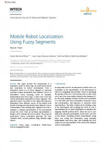
A. Iterative Closest Point Given two sets of 3D points, the iterative closest point algorithm is used to find their relative rotation and translation by registering the two datasets in the same coordinate system. In this algorithm, one dataset is defined as “model” and the other is defined as “data”. The objective is to fit the data points to model points on the overlapping part and find the transformation. As shown in Fig. 7, the points marked in red and green in the left figure are the model and data, respectively, prior to registration. On the right figure, the data points (marked in blue) are transformed and overlap with the model points after carrying out the ICP registration algorithm. The procedure is as follows. • Given a model point, find the corresponding data point with shortest distance.
857
Calculate the displacement of each pair of points using mean square cost function. • Find the rotation and translation between the model and data points based on the previous result. • If the error of the overlapping part of the 3D points is less than a threshold, then stop the process. • Perform the above process iteratively until the error is less than a preset value. Depth measurement using Kinect has the characteristic that the nearby points possess higher accuracy than far away points due to the infrared sensing technique. This property is incorporated in our ICP registration algorithm. Also, since our mobile platform moves on the flat ground plane, it is assumed that the displacement in the vertical direction should be less than a small value. If the ICP iteration have reached but the displacement is larger than the given value, then the ICP iteration will continue until that value is reached or converges. It should be noticed that the vertical displacement cannot be set as zero, since there might be noise or the robot’s movement can lead to vibration, etc. •
Fig. 7 Iterative closest point registration algorithm.
By filtering out the outliers, the rest points are the points of interest and can be used for 3D registration. This can be achieved by using the correspondence information between the color and range images. The 3D coordinates of the color image points are passed to ICP algorithm for registration, as shown in Figure 8(c). The advantage of this color information assisted method is that it can reduce some unwanted point and thus faster in processing. Furthermore, those remaining points are relatively robust, which is less sensitive to large viewpoint changes during the robot’s motion. Consequently, the results are better than the one without color point matching. Fig. 9 shows the flowchart used in our experiment. The ICP registration algorithm is carried out two datasets at a time to estimate the relative motion between two consecutive camera positions. If the result contains any error, it will be passed to the next stage for future rotation and translation estimation. Thus, the error will accumulate during the robot motion. To overcome this problem, we introduce a so-called “keyframe” concept to minimize the overall accumulation error. The keyframe based technique uses certain frame as a reference frame for comparing with all other images. It has the advantage that the rapid error accumulation will not happen in that not every two consecutive image frames are processing for motion estimation. If there is severe error happens for certain displacement calculation, it can be recovered in the future frame. Furthermore, this method is generally faster since there are less frames are used to extract the feature points and for future process.
B. Feature acquisition
(a) SURF keypoint matching.
4000
4000
3000
3000
2000
2000
y
y
If the robot motion is derived only based on the registration of 3D point clouds acquired by the range sensor, it might be inaccurate due to the noise of insufficient overlapping parts. Thus, it is worth investigating by bringing the color information to increase the accuracy of rotation and translation computation. We can use the overlapping parts of two color images, find their correspondences and calculate the robot’s displacement. In recent years, there are many interested point extraction algorithms proposed, including SIFT (Scale Invariant Feature Transform) [10] and SURF (Speedup Up Robust Features) [11] techniques. There also exist other keypoint matching approaches. Juan et al. compared three kinds of feature acquisition methods [15], including SIFT, SURF, and PCA-SIFT. Based on their analysis, we select SURF as for our feature extraction method since it is relatively fast with reasonable good results. After the SIFT or SURF are used to extract the feature points on the color images, correspondence matching is carried out on two consecutive images, as shown in Figure 8(a). Given an image of the current frame, the corresponding points as extracted in the following frame can be obtained. Since it is usually not possible to match all the feature points correctly between the two image frames, we employ the RANSAC (RANdom Sample Consensus) algorithm [16] to filter out the outliers.
1000
1000
0 1500
0 1500 1000
2000 1000
500
0
0 z
1000
2000 1000
500
−500
−2000
x
(b) Before ICP.
0
0
−1000 z
−1000 −500
−2000
x
(c) After ICP.
Fig. 8 Keypoint matching + ICP algorithm.
In most situations, we do not know how many matched feature points are required for motion estimation between two image frames. The depth information acquired by the TOF cameras such as Kinect is also not as accurate as laser range scanners. Thus, it is better to use more matching points to increase the stability of the estimation results. In
858
Fig. 9 The system flowchart of the localization system using an RGB-D camera.
our experiments, we use different thresholds and compare the results. Fig. 10 shows the results obtained from moving a mobile robot along a given path. The figures are the correspondence matching of the keyframe images. The points are the SURF feature points. The estimation between two consecutive positions is connected by a straight line, and the resulting path is shown in the right figure. Fig. 11 Our mobile platform.
to capture the images of the ceiling scenes. In the indoor environment, several markers are attached on the ceiling and their installation positions are known from the environment setting. If there is only one marker pattern seen in the captured image, then it is used to calculate the robot’s location directly. Sometimes there might be several marker patterns seen in the captured image. In such cases, the locations are calculated individually and their average is used as the final result. In this experiment, a mobile platform moves along a U shape path. The estimated path is shown in Fig. 12.
(a) Result 1.
(b) Result 2.
(c) Result 3.
Fig. 12 Experimental results of the mobile platform moving along a U shape path.
B. Localization system using an RGB-D camera (d) Result 4.
Fig. 10 Experimental results of the RGB-D camera based localization system.
IV. EXPERIMENTAL RESULTS In this section, some experimental results are demonstrated with the images captured from the real scenes. We first describe the environment and experimental setup, followed by the results obtained from different environments and settings. A. Localization system using the ceiling landmarks The experiment is carried out on a mobile platform (see Fig. 11), with a camera installed facing upward vertically
In this experiment, the localization system is also implemented on a mobile platform as shown in Fig. 11. A Kinect camera is mounted on the robot for all visual information acquisition. The localization technique is based on the color and depth information captured by the RGB-D camera. The experiments are carried out in an indoor environment. A mobile robot moves along a circular path and returns back to its original location. The path is shown in Fig. 13(a). We chose different threshold values for keyframe extraction for comparison of the associated results. Figs. 13(b), 13(c), and 13(d) show the resulting paths using different threshold values. It can be seen that some sudden changes occurred during the motion, but the path leads to the original location in the end. This is the result of using keyframe for 3D
859
depth in-formation can be obtained. The two kinds of data source can be combined and the extracted feature points can be used for autonomous robot navigation. In this work a commercially available Kinect camera is adopted, it is less expensive but the sensor precision is less than some high-end industrial product. We have demonstrated that the preliminary results are obtained and the proposed method can be extended to more elaborated hardware setting. Since the two localization techniques use different image source, one camera facing upward and the other camera facing forward, it is possible to fuse the information to increase the correctness of robot self-location. This kind of sensor fusion problem is rather difficult and will be investigated in the future research.
3000
3000
2500
2500
2000
2000
1500
1500
1000
1000
500
500
z
z
(a) Motion Path.
0
R EFERENCES
0
−500
−500
−1000
−1000
−1500
−1500
−2000 −3500 −3000 −2500 −2000 −1500 −1000 x
−500
0
500
−2000 −4000 −3500 −3000 −2500 −2000 −1500 −1000 x
1000
(b) Threshold = 30.
−500
0
500
0
500
(c) Threshold = 50. 3000
3000
2500 2000
2000 1500
1000
z
z
1000 0
500 0
−1000
−500 −1000
−2000
−1500 −3000 −4000 −3500 −3000 −2500 −2000 −1500 −1000 x
−500
(d) Threshold = 75.
0
500
−2000 −4000 −3500 −3000 −2500 −2000 −1500 −1000 x
−500
(e) Threshold = 100.
Fig. 13 The actual motion path (Input) and the estimated paths under various threshold values (Output).
data registration and motion parameter estimation. If the consecutive frames are processed sequentially, it is generally not possible to compensate the errors introduced in the frame-by-frame basis. V. CONCLUSION In the paper, two different approaches for autonomous robot localization are proposed. The first approach can do global localization while the second is similar to visual odometry(local localization). In both approaches, the positions are calculated from the features of the images captured from the real scene. There is no need for any prior object feature extraction and training, etc. The underlying technologies of these two approaches are not the same, so they have their own advantages and drawbacks. The ceiling landmark based localization approach tries to identify the pre-defined and pre-installed landmark from the ceiling images. As long as the landmarks can be observed by the camera, the robot location can be uniquely determined. Thus, the autonomous navigation can be achieved in any environment by properly setting up the ceiling landmark patterns. Using the RGB-D camera, the color images and
[1] M. S. Grew-al and A. P. Andrew, Kalman Filtering : Theory and Practice. Wiley-Interscience, 2 ed., Jan. 2001. [2] Kalman, Rudolph, and Emil, “A new approach to linear filtering and prediction problems,” Transactions of the ASME-Journal of Basic Engineering, vol. 82, no. Series D, pp. 35-45, 1960. [3] Z. Zhang, “Iterative point matching for registration of free-form curves and surfaces,” Int. J. Comput. Vision, vol. 13, pp. 119-152, October 1994. [4] R. Negenborn, Robot Localization and Kalman Filters - On fnding your position in a noisy world, M.S. Thesis, Utrecht University, Sep. 2003. [5] A. Rituerto, L. Puig, and J. J. Guerrero, “Visual slam with an omnidirectional camera,” in Proceedings of the 20th International Conference on Pattern Recognition, ICPR’10, Washington, DC, USA, pp. 348-351. [6] P. Henry, M. Krainin, E. Herbst, X. Ren, and D. Fox, “Rgb-d mapping : Using depth cameras for dense 3d modeling of indoor environments,” In RGB-D: Advanced Reasoning with Depth Cameras Workshop in conjunction with RSS, vol. 1, no. c, pp. 9-10, 2010. [7] V. Castaneda, D. Mateus, and N. Navab, “Slam combining tof and highresolution cameras,” in Proceedings of the 2011 IEEE Workshop on Applications of Computer Vision (WACV), WACV’11, (Washington, DC, USA), pp. 672-678, IEEE Computer Society, 2011. [8] F. Fraundorfer, C. Wu, and M. Pollefeys, “Combining monocular and stereo cues for mobile robot localization using visual words,” in Proceedings of the 2010 20th International Conference on Pattern Recognition, ICPR’10, (Washington, DC, USA), pp. 3927-3930, IEEE Computer Society, 2010. [9] D. Chen and G. Zhang, “A new sub-pixel detector for x-corners in camera calibration targets,” in International Conference in Central Europe on Computer Graphics and Visualization, pp. 97-100, 2005. [10] D. G. Lowe, “Object recognition from local scale-invariant features,” in Proceedings of the International Conference on Computer VisionVolume 2 - Volume 2, ICCV’99,(Washington, DC, USA), pp. 11501157, IEEE Computer Society, 1999. [11] H. Bay, A. Ess, T. Tuytelaars, and L. Van Gool, “Speeded-up robust features (surf),” Comput. Vis. Image Underst., vol. 110, pp. 346-359, June 2008. [12] J. H. Zhou and H. Y. Lin, “A Self-Localization and Path Planning Technique for Mobile Robot Navigation,” 2011 World Congress on Intelligent Control and Automation (WCICA 2011), Taipei, Taiwan, June 21-25, 2011. [13] A. Murillo, J. Guerrero, and C. Sagues, “Surf features for efficient robot localization with omnidirectional images,” in Robotics and Automation, 2007 IEEE International Conference on, pp. 3901-3907, april 2007. [14] C. Harris and M. Stephens, “A combined corner and edge detector,” in Proceedings of the 4th Alvey Vision Conference, p. 147-151, 1988. [15] L. Juan and O. Gwon, “A comparison of SIFT, PCA-SIFT and SURF,” International Journal of Image Processing (IJIP), vol. 3, no. 4, pp. 143152, 2009. [16] M. A. Fischler and R. C. Bolles, “Random sample consensus: a paradigm for model fitting with applications to image analysis and automated cartography,” Commun. ACM, vol. 24, pp. 381-395, June 1981.
860