May 7, 2008 - We thank Georgia Tech, its Sony-Toshiba-IBM. Center of Competence, and ... High Performance Computing (HiPC), Lecture Notes in Computer ...
Cell-SWat: Modeling and Scheduling Wavefront Computations on the Cell Broadband Engine ∗
Ashwin M. Aji, Wu-chun Feng, Filip Blagojevic and Dimitrios S. Nikolopoulos Center for High-End Computing Systems Virginia Tech 2202 Kraft Drive Blacksburg, VA 24060
{aaji,feng,filip,dsn}@cs.vt.edu ABSTRACT
General Terms
This paper presents and evaluates a model and a methodology for implementing parallel wavefront algorithms on the Cell Broadband Engine. Wavefront algorithms are vital in several application areas such as computational biology, particle physics, and systems of linear equations. The model uses blocked data decomposition with pipelined execution of blocks across the synergistic processing elements (SPEs) of the Cell. To evaluate the model, we implement the Smith-Waterman sequence alignment algorithm as a wavefront algorithm and present key optimization techniques that complement the vector processing capabilities of the SPE. Our results show perfect linear speedup for up to 16 SPEs on the QS20 dual-Cell blades, and our model shows that our implementation is highly scalable for more cores, if available. Furthermore, the accuracy of our model is within 3% of the measured values on average. Lastly, we also test our model in a throughput-oriented experimental setting, where we couple the model with scheduling techniques that exploit parallelism across the simultaneous execution of multiple sequence alignments. Using our model, we improved the throughput of realistic multisequence alignment workloads by up to 8% compared to FCFS (first-come, first-serve), by trading off parallelism within alignments with parallelism across alignments.
Design, Experimentation, Performance, Theory
Categories and Subject Descriptors C.1.4 [Processor Architectures]: Other Architecture Styles—Heterogeneous (hybrid) systems; C.4 [Performance of Systems]: [Modeling techniques]; J.3 [Life and Medical Sciences]: [Biology and genetics] ∗Institute of Computer Science (ICS) Foundation of Research and Technology Hellas (FORTH) P.O. Box 711 00, Heraklion, Crete, GREECE
Permission to make digital or hard copies of all or part of this work for personal or classroom use is granted without fee provided that copies are not made or distributed for profit or commercial advantage and that copies bear this notice and the full citation on the first page. To copy otherwise, to republish, to post on servers or to redistribute to lists, requires prior specific permission and/or a fee. CF’08, May 5–7, 2008, Ischia, Italy. Copyright 2008 ACM 978-1-60558-077-7/08/05 ...$5.00.
Keywords Wavefront algorithms, Smith-Waterman, Cell Broadband Engine
1.
INTRODUCTION
The accelerated dissemination of the Cell Broadband Engine (Cell/BE), a general-purpose high-performance processor, motivates users to rethink some of the fundamental principles of parallel programming models and methodologies. Architectural properties such as heterogeneous cores, multiple layers of thread and data parallelism, software-managed memory hierarchies, and disjoint address spaces have implications on both algorithmic techniques for parallelizing computation and system software for orchestrating parallel execution. While many recent studies have explored the potential of the Cell/BE as a compute engine and developed optimization techniques and high-level programming interfaces for taming Cell’s heterogeneity [4, 8, 10, 16, 22], programmers are still in need of systematic methodologies, models, and patterns for high-performance programming on the Cell. This paper contributes and evaluates a model and a methodology for implementing parallel wavefront algorithms on the Cell/BE. Wavefront (or systolic) algorithms expose parallelism from computations with recurrences, by breaking up the computations into segments and pipelining the execution of the segments across processors. Wavefront algorithms are of paramount importance in several application areas, ranging from particle physics to systems of linear equations to motion planning to computational biology [14]. We present a comprehensive model for tiled wavefront algorithms for the Cell/BE that can optimally guide the selection of tile size, the scheduling of tiles on the accelerator cores of the processor (SPEs), and the scheduling of multiple simultaneous tiled wavefront computations via spatial partitioning of the SPEs in order to improve overall throughput. We also present and evaluate an implementation of the Smith-Waterman algorithm on the Cell/BE. SmithWaterman is a local sequence alignment method which guarantees optimality but at the cost of high (quadratic) time and space complexity.
Our implementation of Smith-Waterman extends and complements earlier efforts to vectorize the algorithm in SIMD-enabled accelerators (including FPGAs [21], GPUs [15], and conventional processors with SIMD extensions [18]), with a wavefront execution scheme that exploits multiple accelerators simultaneously. We leverage our model to optimize the heterogeneous parallelization, data localization and scheduling of individual Smith-Waterman sequence alignments on the Cell/BE. Thereafter, we use our model to improve the simultaneous execution of multiple Smith-Waterman alignments on multi-processor Cell-based systems, under the experimental conditions used in practice by computational biologists. In addition, we model the execution of the tiled wavefront Smith-Waterman algorithm on the Cell/BE with an absolute error as low as 3% on average. Our model-driven implementation of Smith-Waterman on Cell/BE achieves linear 16-fold acceleration of Smith-Waterman on two Cell/BEs with 16 synergistic processing elements (SPEs) in total, compared to the optimized implementation of Smith-Waterman on a 2.8-GHz dual-core Intel processor. Finally, we also improve the overall throughput of multiple Smith-Waterman sequence alignments by 8% on dual-Cell blades, by trading off parallelism within local sequence alignments with parallelism across sequence alignments. The rest of this paper is organized as follows: Section 2 outlines the Cell/BE architecture and our experimental setting. Section 3 presents our model of wavefront algorithms for the Cell/BE and architectures with asymmetric cores. Section 4 presents our implementation of Smith-Waterman, following the execution model detailed in Section 3. Section 5 presents our experimental analysis. Section 6 discusses related work, and Section 7 concludes the paper.
2.
EXPERIMENTAL PLATFORM
The Cell/BE is a heterogeneous processor that integrates a total of 9 cores: a two-way SMT PowerPC core (the Power Processing Element or PPE), and 8 tightly coupled SIMD-based processors (the Synergistic Processing Elements SPEs) [9]. The components of the Cell processor are connected via a high bandwidth Element Interconnect Bus (EIB). The EIB is a four-ring structure, running at half the processor frequency (1.6 GHz) and capable of transmitting 96 bytes per cycle for a maximum theoretical memory bandwidth of 204.8 gigabytes/second. The EIB can support more than 100 outstanding DMA requests. The PPE is a 64-bit SMT processor running the PowerPC instruction set architecture (ISA) with vector/SIMD multimedia extensions. The PPE boasts two levels of on-chip cache, L1-I and L1-D with a capacity of 32 KB each, and L2 with a capacity of 512 KB. Each SPE has two main components, the Synergistic Processor Unit (SPU) and the Memory Flow Controller (MFC). The SPU has 128 registers, each 128 bits wide, and 256 KB of software-managed local store. Each SPU can access only local store with direct loads and stores and off-chip memory or memory-mapped local stores of other SPUs through DMAs. The PPE can also access the local stores of the SPUs via DMAs. The SPU has a different ISA than the PPE and leverages vector execution units to implement Cell-specific SIMD intrinsics on the 128-bit wide registers. The MFC serves DMAs from and to the local stores and supports DMA lists that enable triggering of up to 2048 DMA transfers with
a single command. The MFC enables complete overlap of DMA latency with computation. Single-precision floating point (FP) operations are dualissued and fully pipelined on the SPEs, whereas doubleprecision floating point operations have a 13-cycle latency with only the last 7 cycles pipelined. No other instructions can be issued in the same instruction slot with doubleprecision floating point instructions and no instructions of any kind are issued for 6 cycles after a double-precision instruction is issued. These limitations severely impact the performance of Cell/BE in double-precision floating point arithmetic. The theoretical peak performance of the Cell processor with all eight SPUs active and fully pipelined double-precision FP operation is only 21.03 Gflops. With single-precision FP, the Cell/BE is capable of a peak performance of 230.4 Gflops [7]. In this study, we used a QS20 dual-Cell blade, part of the Cellbuzz cluster located at Georgia Tech. Each Cell processor on the QS20 blade runs at 3.2 GHz. The blade has 1 GB of XDRAM, which is organized as a NUMA shared memory distributed evenly between the two processors (i.e., 512 MB attached to each processor with longer latency for a processor to access the XDRAM module of the other processor).
3.
GENERAL MODEL OF WAVEFRONT ALGORITHMS ON THE CELL/BE
The wavefront algorithm is an important pattern utilized in a variety of scientific applications, including particle physics, motion planning, and computational biology [14]. Computation proceeds like a wavefront filling a matrix, where each cell of the matrix is evaluated based on the values of cells computed earlier. The algorithm advances through the matrix by computing all anti-diagonals starting from the northwest corner, as shown in Figure 1(a). The computation carries dependencies across anti-diagonals, that is, each element of the matrix depends on its respective northern, western, and northwestern neighbors, as shown in Figure 1(b). In this study, we focus on programming models which enable efficient parallel execution of wavefront algorithms on the Cell/BE. As an example wavefront algorithm, we consider the Smith-Waterman (SWat) algorithm, which performs optimal local genomic sequence alignment [20].
NW
N
W (a)
(b)
Figure 1: A general wavefront algorithm (a) and its dependencies (b). While consecutive anti-diagonals are dependent, the cells lying on the same anti-diagonal are independent and can be processed in parallel. Processing individual matrix elements in parallel incurs high communication overhead which can be reduced by grouping matrix cells into large,
computationally-independent blocks, which are more suitable for parallel processing. This common optimization strategy is outlined in Figure 2. We refer to each block of matrix cells as a tile. The coarsened basic unit of work does not change the properties of the wavefront algorithm – the algorithm advances through the matrix by computing anti-diagonals which are composed of multiple tiles. The most important aspects of the wavefront algorithm are tile computation and communication among processes which perform computation on different tiles. We describe each of the two steps and their implementation on the Cell/BE in more detail in Sections 3.1 and 3.2
northwest neighbor. The same process repeats until the algorithm reaches the right edge of the matrix, after which the computation continues in the next block-row. The matrix is split into multiple block-rows and possible underutilization of the Cell processor might occur only in the last row, if the height of the row is smaller than the number of SPEs. This can easily be avoided by resizing the tiles in the last block-row. X S tiles
S1
t1
t2
t3
S2
t2
t3
t4
S3
t3
t4
t5
‘m’ block rows
Computation overlap
Y
Block Row
n tiles
Figure 3: Matrix divided into block rows. S1
Figure 2: Tiled wavefront.
3.1
Tile Computation
The Cell/BE contains multiple accelerator cores capable of performing independent asynchronous computation. To map the wavefront algorithm to the Cell/BE we assign independent tiles for processing on different SPEs. Assuming the matrix is divided in square tiles, as presented in Figure 2, the execution starts by processing tile t1 . Due to the computational dependencies across anti-diagonals, the tiles lying on the anti-diagonal t2 can be processed only after t1 has been computed. Although the described behavior limits the amount of parallelism exposed by the application, the utilization of the SPE cores increases as the algorithm advances through the matrix. Starting with the anti-diagonal t8 , the number of tiles available for parallel processing is equal to or exceeds the number of SPEs on a single Cell chip, and all SPEs can be used for tile processing. While different scheduling strategies can be used for assigning the units of work to SPEs, we focus on predetermined tile-SPE assignment in this study. Our scheduling scheme achieves perfectly balanced SPE work assignment, while at the same time enables complete utilization of the Cell chip. We change the algorithm computation direction, and instead of computing entire anti-diagonals, the algorithm advances through the block-rows, as shown in Figure 3. The height of each block-row is equal to the total number of SPEs. For anti-diagonals which contain more tiles than the number of available SPEs, the part of the anti-diagonal which belongs to the block-row is computed, and the computation shifts to the next anti-diagonal. Note that this is legal execution since the computation of each tile depends on its north, west, and
While working on an anti-diagonal in a block-row, each SPE is assigned a single tile. Along with the algorithm, the SPEs advance through the block-row towards the right edge of the matrix. After reaching the edge, each SPE continues processing the tiles contained in the next block-row. No two SPEs reach the edge of the matrix at the same time, which causes computation overlap of consecutive block-rows, which is shown in Figure 3 (processing the end of the first block row overlaps with the beginning of the second block row). Simultaneous processing of different block-rows enable high utilization of the Cell processor – the idle SPEs are assigned work units from the next block-row.
3.2
Communication
Communication patterns that occur during the tile computation are shown in Figure 4. We describe step-by-step communication-computation mechanism performed by each SPE while processing a tile: 1. To start computing a tile, an SPE needs to obtain boundary data from its west, north, and northwest neighbor. The boundary elements from the northern neighbor are fetched to the local storage from the local storage of the SPE which was processing the northern neighbor. The boundary elements of the west neighbor do not need to be fetched due to the fact that each SPE advances through a tiled row, and therefore each SPE already contains the required data. The necessary boundary elements of the northwestern neighbor also reside in the local storage of the SPE which processed the northern neighbor, and are fetched along with the boundary elements from the northern neighbor. 2. In the second step, the SPE proceeds with the tile computation.
S(Nspe ), where Nspe is the number of available SPEs. From the above discussion, we represent the total time T from Equation (1) as:
North Tile
X
X
X
X
X
X
DMA
X
X
X
X
X X
Buffer copy
X
X
X
X
DMA tile to main memory
T = (TT ile + TDM A ) · [(m × n) + S(Nspe )]
X
We can further decompose m as: m=
X X
X
X
X
X ‘Ready’ message
West Tile
East Tile
n=
Figure 4: Computation-communication pattern as seen from a single tile.
3. Finally, the SPE moves the tile to main memory for post-processing and notifies the SPE which works on the south neighboring tile that the boundary elements are ready for transfer. The above steps describe the processing of non-boundary tiles. Boundary conditions can be easily checked and the redundant steps can be avoided.
Wavefront Model for the Cell/BE
To capture the performance of the wavefront algorithm on the Cell/BE, we developed an analytical model capable of accurately predicting the total execution time of the algorithm. As an input, the model takes several application specific parameters and estimates execution time on a variable number of cores. We start the discussion about the model by introducing the following equation: T
= TF + Tserial
Y TSize · Nspe
(3)
where Y represents elements (not tiles) in the y-dimension of the matrix, TSize represents the size of a tile, and Nspe is again the number of available SPEs (equal to the height of the block-row). Also, we can decompose n as:
South Tile
3.3
(2)
(1)
In Equation (1), T represents the total time taken by the algorithm, TF is the time the algorithm uses to fill the matrix, and Tserial is the time taken by the inherently sequential part of the algorithm. If we denote the time needed to compute one tile as TT ile and the time used to fetch and commit the data necessary for tile computation as TDM A , then the total time spent processing a single tile can be represented as TT ile + TDM A . Since all elements of a single anti-diagonal (in a block-row) are processed in parallel, the time to process the entire antidiagonal (in a block-row) can also be represented as TT ile + TDM A . The total number of tiled anti-diagonals should be carefully counted, since it involves overlaps of anti-diagonals between adjacent block rows. By inspecting Figure 3, we estimate the total number of anti-diagonals to be (n · m) + S, where m represents the total number of block-rows, n represents the number of anti-diagonals per block-row, and S is the number of anti-diagonals containing less tiles than the number of SPEs and therefore their processing does not utilize the entire Cell chip. In Figure 3, these diagonals are represented in the upper left corner of the matrix. S depends on the number of SPEs, and therefore we can denote it as
X TSize
(4)
where X represents elements (not tiles) in the x-dimension of the matrix, Combining Equations (1), (2), (3), and (4), we derive the final modeling equation: � � X ·Y T = (TT ile + TDM A ) · + S(Nspe ) + Tserial 2 TSize · Nspe (5) To employ the model as a run-time tool capable of determining the most efficient execution configuration, we need to estimate all parameters included in the model. The parameters TT ile and TDM A need to be measured before they can be plugged into the model. The measurement can be performed during a short sampling phase, which would occur at the beginning of the program execution or via offline microbenchmarks. By knowing TT ile and TDM A for a single tile size (Tsize ), we can accurately estimate the same parameters for any tile size. This is due to the fact that each tile is composed of the matrix cells that require equal amount of processing time. X and Y depend on the input data set and can be determined statically. Nspe , S(Nspe ) and Tsize are related to the number of SPEs used for parallelization and the tile size. These parameters can iterate trough different values, and those that provide the most efficient execution will be used for the algorithm execution. Parameter Tserial does not influence the parallel execution of the program, and we can disregard this parameter while searching for the most efficient parallel configuration.
4.
MODEL EVALUATION: SMITHWATERMAN (SWAT) ALGORITHM
To evaluate our tiled wavefront model, we use the SmithWaterman (SWat) algorithm. The algorithm is introduced in Section 4.1 and implementation details of parallelizing SWat are discussed in Section 4.2. Results and evaluation of our model are discussed in Section 5.
4.1
The Algorithm
The Smith-Waterman algorithm is a well-known, dynamic-programming algorithm for performing optimal local sequence alignment, i.e., determining similar regions between two nucleotide or protein sequences. Instead of looking at the overall sequence (as in the case of global alignment), the Smith-Waterman algorithm compares segments of all possible lengths and optimizes the similarity measure, which is termed as the alignment score of the sequences.
This is followed by outputting the highest scoring local alignment. The algorithm can be partitioned into two phases: (1) matrix filling and (2) backtracing. • Matrix filling: The optimal alignment score is computed by filling out a dynamic programming matrix, starting from the northwest corner and moving towards the southeast corner, following the wavefront pattern. The matrix is filled based on a scoring system, which is composed of two subsystems:
NW
– The substitution matrix, M : Each entry in the substitution matrix, M (i, j), indicates the score of aligning the characters i and j. If M (i, j) is positive, then there is a match between i and j, and the score is referred to as a reward. A higher positive score indicates a better match. If M (i, j) is negative, then it is a mismatch between i and j, and the score is a penalty.
W N
Figure 5: 3D dependencies
– The gap-scoring scheme: Gaps are introduced between the amino acid or nucleotide residues (a single character in a sequence) so that similar characters get aligned to potentially increase the alignment score. These gaps are usually denoted by a ‘–’ in the output alignment. They are considered to be a type of a mismatch and incur some penalty. We consider the system with affine gap penalties which means that there are two types of gap penalties: 1. Gap-open penalty (o): This is the penalty for starting (or opening) a gap in the alignment 2. Gap-extension penalty (e): This is usually a less severe penalty than the gap-open penalty. It is imposed for extending a previously existing gap in the alignment by one unit. Thus, if there are k consecutive gaps in an alignment, then the total gap penalty incurred by that gap is o + k × e. The recursive data dependence of the elements in the dynamic-programming matrix can be explained by the following equations: DPN [i − 1, j] DPW [i − 1, j] + o DPN [i, j] = e + max DP N W [i − 1, j] + o DPN [i, j − 1] + o DPW [i, j − 1] DPW [i, j] = e + max DP N W [i, j − 1] + o
(6)
(7)
DPN [i − 1, j − 1] DPW [i − 1, j − 1] DPN W [i, j] = M (Xi , Yj )+max DP N W [i − 1, j − 1] (8) Equations (6), (7), and (8) indicate the presence of three weighted matrices and also imply a threedimensional (3D) dependency among the elements of the matrix as shown in Figure 5. The elements of
the matrix DPN are dependent only on the northern neighbors of the three available weighted matrices. Similarly, DPW and DPN W have elements that depend only on their respective western and northwestern neighbors of the available three weighted matrices, thereby maintaining the wavefront pattern. • Backtracing: This stage of the algorithm yields the highest scoring local alignment. The backtrace begins at the matrix cell that holds the optimal alignment score and proceeds in a direction opposite to that of the matrix filling, until a cell with score zero is encountered. The path traced by this operation generates the alignment.
4.2
Implementation and Optimizations
We profiled the serial SWat code on a general- purpose CPU using gprof and found that 99.9% of the time is spent in the matrix filling part, therefore this part became the obvious choice for parallelization. The computation and communication patterns of Cell-SWat are similar to what was discussed in section 3, since our implementation follows the tiled wavefront approach. The implementation and optimization details that are specific to Cell-SWat are discussed in this section. Tile representation: Each tile is physically stored in memory, as a 1D array, by storing adjacent anti-diagonals next to each other. This is depicted in Figure 6. This arrangement makes it easier to perform vector operations on the tile by taking one anti-diagonal at a time. Vectorization of the tile for the SPE: We assign each tile to execute on individual SPEs. To extract the true potential of the SPEs, the data has to be vectorized before being operated upon. The vectorization process that we follow is described by Figure 7. A two-dimensional (2D) representation is shown in the figure (instead of 3D) for the sake of simplicity. During a tile vectorization process, we process one anti-diagonal at a time following the wavefront pattern. To effectively utilize the SIMD capabilities
C
G
A
T
35
0
0
0
0
0
30
G
0
0
3
1
0
A
0
0
1
6
4
15
Matrix Filling
A
0
0
0
4
5
10
Total Time
7
5
T
0
0
0
2
Speedup
25 20
0 1 2 3 4 5 6 7 8 9 10 11 12 13 14 15 16 Number of SPEs
0 0 0 0 0 0 0 0 3 0 0 0 1 1 0 0 0 6 0 0 4 4 2 5 7
(a) Figure 6: Tile representation in memory. 12
G
G
A
T
T
0
0
0
0
0
T
0
0
0
0
0
9
G
0
5
5
0
3
A
0
0
2
5
A
0
0
2
T
0
0
T
0
C 0
8 6 Backtrace 4
Matrix Filling
2 0
Serial computation
0
Time (seconds)
10
Figure 7: Tile vectorization.
of the SPE, the anti-diagonal must be divided into as many vectors as possible. The number of elements on the antidiagonal keeps changing for every anti-diagonal and cannot be perfectly partitioned into vectors in some cases. In these cases, the remainimg elements undergo a serial computation. Upon vectorization, we obtained the speedup and execution time curves shown in Figure 8(a) and (b), respectively. These timings were recorded for input sequence lengths of 8 KB. Figure 8 indicates reduced speedup when the number of SPEs exceeds 6. The reason is the backtrace phase, which is completed solely on the PPE and does not depend on the number of SPEs. The sequential backtrace calculation on the PPE is the next bottleneck for optimization. The backtrace optimization: The backtrace begins at the matrix cell that holds the largest alignment score; therefore, a find max operation is needed. Initially, our implementation executed this function on the PPE after the entire matrix was filled up. To reduce the high PPE overhead caused by the backtrace operation, we optimized find max by parallelizing it across SPEs. The local optimum score calculated by each SPE is passed on to the PPE at the end of the ma-
1
2
3
4
5
6
7
8
9 10 11 12 13 14 15 16
Number of SPEs
(b) Figure 8: Speedup (a) and timing (b) charts before optimizing the backtrace operation.
trix filling phase. From this data, the PPE calculates the overall optimum score by performing at most S if checks, where S is the number of SPEs used. This optimization had a considerable impact on the achieved speedups (as shown in Figure 9).
5.
RESULTS
We present results from experiments on a single, dedicated dual-Cell/BE QS20 blade. We conducted these experiments by aligning sequences of realistic sizes as are currently present in the NCBI Genbank nucleotide (NT) database. There are approximately 3.5 million sequences in the NT database. Of those, approximately 95% are 5 KB in size or less [11]. For the tests, we chose eight randomly generated sequence pairs of sizes varying from 1 KB to 8 KB in increasing steps of 1 KB, thus covering most of the realistic sequence sizes. We randomly generated the input sequences because the complexity of the Smith-Waterman algorithm is dependent only on the sequence length and not on the sequence contents. We repeated the tests for the above sequence lengths by varying the number of SPE threads from 1 to 16 to test the scalability of our implementation on up to two fully utilized Cell processors. To measure the effect of tile granularity on the execution times, we repeated all of the above experiments for tile sizes of 8, 16, 32 and 64
25
20
20
15
15
Speedup
Speedup
25
Matrix Filling
10
Tile Size = 64 Tile Size = 32
10
Tile Size = 16
Total time 5
5
0
0
Tile Size = 8
1 2 3 4 5 6 7 8 9 10 11 12 13 14 15 16
1 2 3 4 5 6 7 8 9 10 11 12 13 14 15 16
Number of SPEs
Number of SPEs
Figure 10: The obtained speedup for input sequences of length 8KB. The number of SPEs varies from 1 to 16.
(a) 7
Time (seconds)
6 5
5.2
4 3
Backtrace
2
Matrix Filling
1 0 1
2
3
4
5
6
7
8
9 10 11 12 13 14 15 16
Number of SPEs
(b) Figure 9: Speedup (a) and timing (b) charts after optimizing the backtrace operation.
elements. To measure the speedup of our implementation, we executed the serial version of Smith-Waterman on a machine with a 2.8-GHz dual-core Intel processor and 2-GB memory, and we used one of the two cores present on the chip. We believe that using the Intel processor as a basis for calculating speedup on the Cell is more realistic than using the PPE core, which has very limited computational capacity compared to the SPEs. Using the PPE core as a basis for speedup calculation would only inflate the results with not much added value.
5.1
7
Time (seconds)
6 5 4 3
Practice
2
Theory
1 0
Speedup
Figure 10 illustrates the achieved speedup with different numbers of SPEs. Similar curves were observed for all eight sequence sizes. The speedup curves indicate that our algorithm delivers perfect linear speedup for up to 16 SPEs, irrespective of the tile size, and it is highly scalable for more cores if they are available on the chip. The figure also shows that as the tile size increases, more speedup is achieved. This is because more data is locally available for each SPE to work upon, and there is less communication overhead between the SPEs. We were not able to choose a tile size of more than 64 elements because the memory required to work on a single tile exceeded the capacity of the local store of the SPE.
Model Verification
To verify our model, we initially experimentally measured Ttile , TDM A and Tserial by varying the other parameters of Equation (5). We chose an example sequence pair of 8KB in size and tile size of 64 for this experiment. The measured values for this configuration were Ttile = 0.00057s, TDM A = 10−6 s and Tserial = 0.015s. By varying S from 1 to 16, we generated a set of theoretically estimated execution times. The theoretical estimates from our wavefront model was then compared to the actual execution times, as seen in Figure 11. Similar results were observed for all the other sequence sizes and tile sizes as well. This shows that our model estimates accurately the execution time taken to align two sequences of any size, using any number of SPEs or any tile size. The model error is within a range of 3% on average.
1
2
3
4
5
6
7
8
9 10 11 12 13 14 15 16
Number of SPEs
Figure 11: Chart showing theoretical timing estimates of our model (labeled theory) against the measured execution times (labeled practice).
5.3
Sequence Throughput
We now consider a realistic scenario for the use of SmithWaterman by computational biologists, where multiple pairwise sequences need to be aligned. Using our model, we
target achieving higher sequence throughput, i.e align more sequence pairs per unit time. The straightforward approach is to align the sequence pairs, one pair at a time, in a firstcome-first-served (FCFS) fashion – where each alignment uses all 16 SPEs. By using all the 16 SPEs for one alignment, we achieve maximum parallelism within each sequence alignment. However, we can also achieve parallelism across sequence alignments where many pairs are aligned at the same time, and each pair uses less than 16 SPEs. A simple experiment was conducted by executing 2, 4 and 8 pairs of sequences in parallel, and this was compared against the FCFS approach. The results are as shown in Figure 12. The results indicate the processing multiple sequences in parallel achieves higher throughput than processing each sequence separately using all available SPEs. More specifically, sacrificing some parallelism within each sequence alignment can be traded off profitably for increasing the number of sequence alignments processed in parallel, via spatial partitioning of the Cell SPEs. We can thus create a schedul-
0.9 0.8 Time (seconds)
0.7 0.6 0.5 0.4
FCFS execution
0.3
Parallel execution
0.2 0.1 0 2
4
8
Number of sequence pairs
Figure 12: Comparison of FCFS execution and parallel strategies where 2, 4, and 8 pairs of sequences are processed in parallel. ing algorithm for achieving sequence throughput by deciding the set of sequence pairs that have to executed in parallel. To test the described strategy, we obtained the distribution of sequences in the nucleotide (NT) database for sequence lengths of less than 8 KB. We generated 100 sequence pairs based on the NT distribution, thereby imitating a realistic workload. We follow a static scheduling scheme where equal-sized sequence pairs are taken in batches and executed in parallel, provided that they not overflow the memory. While this scheme is by no means optimized, it can show the potential of our model by taking into account the estimated speedup and scalability slopes for each sequence length, while scheduling multiple alignments. We evaluate the tradeoffs of the FCFS approach versus our scheduling approach for the experimental work set and the results are shown in the Table 1. The analytical model we developed and described in Section 3 can be used to analyze the different tradeoffs between FCFS and the various sequence scheduling policies accurately. In the case of our static scheduling scheme, we are able to improve throughput compared to FCFS and execution of alignments at the maximum level of available concurrency by 8%. In our future work, we plan to employ the model and investigate optimal
FCFS execution 26.67792s
Parallel execution 24.552805s
Table 1: Performance comparison between the FCFS approach and parallel execution on a realistic data set. scheduling strategies that would maximize the throughput of the algorithm.
6.
RELATED WORK
Many recent research efforts explored application development, optimization methodologies and new programming environments for the Cell/BE. In particular, recent studies investigate Cell/BE-specific implementations of applications including particle transport codes [17], numerical kernels [1], FFT [2], irregular graph algorithms [3], computational biology [19], sorting [12], query processing [13], and data mining [6]. Our research departs from these earlier studies in that it models and optimizes a parallel algorithmic pattern that is yet to be explored thoroughly on the Cell/BE, namely tiled wavefront algorithms. The work closest to our research is a recent parallelization and optimization of the wavefront algorithm used in a popular ASCI particle transport application, SWEEP3D [17], on the Cell/BE. Our contribution differs in three aspects. First, we consider inter-tile parallelism during the execution of a wavefront across the Cell SPEs in order to cope with variable granularity and degree of parallelism within and across tiles. Second, we provide an analytical model for tiled wavefront algorithms to guide parallelization, granularity selection, and scheduling for both single and multiple wavefront computations executing simultaneously. Third, we consider throughput-oriented execution of multiple wavefront computations on the Cell/BE, which is the common usage scenario of these algorithms in the domain of computational biology. Our research also parallels efforts for porting and optimizing key computational biology algorithms, such as phylogenetic tree construction [5] and sequence alignment [19]. The work of Sachdeva et. al [19] relates to ours, as it explores the same algorithm (Smith-Waterman), albeit in the context of vectorization for SIMD-enabled accelerators. We present a significantly extended implementation of SmithWaterman that exploits pipelining across multiple accelerators in conjunction with vectorization and optimizes task granularity and multiple query execution throughput on the Cell. We also extend this work through a generic model of wavefront calculations on the Cell/BE, which can be applied to a wide range of applications using dynamic programming for both performance-oriented and throughput-oriented optimization. Recently proposed programming environments (languages and runtime systems) such as Sequoia [10], Cell SuperScalar [4], CorePy [16] and PPE-SPE code generators from single-source modules [8, 22], address the problem of achieving high performance on the Cell with reduced programming effort. Our work is oriented towards simplifying the effort to achieve high performance from a specific algorithmic pattern on the Cell/BE and is orthogonal to related work on programming models and interfaces. An interesting topic for future exploration is the expression of wavefront algorithms with high-level language constructs, such as those provided by Sequoia and CellSs, and techniques for automatic opti-
mization of key algorithmic parameters in the compilation environment of high-level parallel programming languages.
7.
CONCLUSION
This paper presented techniques to model, optimize, and schedule tiled wavefront computations on the Cell Broadband Engine. Our model was designed to guide the optimization of data staging and scheduling of wavefront computations on heterogeneous multi-core processors. We have deployed the model in Smith-Waterman, an important algorithm for optimal local sequence alignment, and we stresstested our modeling methodology and our optimizations both in terms of accelerating isolated sequence alignments as well as in a throughput-oriented experimental setting, where we couple our model with dynamic space sharing of the SPE cores of the Cell processor and trade intra-sequence parallelism for inter-sequence parallelism. We achieved linear speedup with respect to the number of Cell SPEs for Smith-Waterman on IBM QS20 Cell blades, using a 2.8 GHz Intel dual-core processor as a basis for comparison. We obtained this result via a combination of optimization of the tile size of wavefront computations on SPEs, optimization of data layout for vectorization, and acceleration of reduction through the SPEs. We have also been able to improve the throughput of realistic multi-sequence alignment workloads by up to 8% compared to FCFS, by trading off parallelism within sequence alignments with parallelism across sequence alignments, using a static spacesharing methodology and our model to assess the trade-off. This result can be improved with dynamic space-sharing schemes, which we intend to explore in future work. We also intend to investigate the integration of our SWat implementation of Cell into sequence alignment toolkits and extend our modeling and implementation methodologies for SWat and wavefront algorithms onto clusters of heterogeneous multi-core nodes by introducing an outer layer of MPI parallelism in our wavefront implementations.
[4]
[5]
[6]
[7]
[8]
[9]
[10]
[11]
[12]
Acknowledgment This research is supported by the NSF (grants IIP-0804155, CCF-0346867, CCF-0715051, CNS-0521381, CNS-0720673, CNS-0709025, CNS-0720750), the DOE (grants DE-FG0206ER25751, DE-FG02-05ER25689), and by IBM through a pair of IBM Faculty Awards (VTF-873901 and VTF874197). We thank Georgia Tech, its Sony-Toshiba-IBM Center of Competence, and NSF for the Cell/BE resources that have contributed to this research.
8.
[13]
[14]
REFERENCES
[1] S. Alam, J. Meredith, and J. Vetter. Balancing Productivity and Performance on the Cell Broadband Engine. In Proc. of the 2007 IEEE Annual International Conference on Cluster Computing, September 2007. [2] D. Bader and V. Agarwal. FFTC: Fastest Fourier Transform for the IBM Cell Broadband Engine. In Proc. of the 14 th IEEE International Conference on High Performance Computing (HiPC), Lecture Notes in Computer Science 4873, 2007. [3] D. Bader, V. Agarwal, and K. Madduri. On the Design and Analysis of Irregular Algorithms on the
[15]
[16]
[17]
Cell Processor: A Case Study of List Ranking. In Proc. of the 21st International Parallel and Distributed Processing Symposium, pages 1–10, 2007. P. Bellens, J. P´erez, R. Badia, and J. Labarta. Memory - Cellss: A Programming Model for the Cell BE Architecture. In Proc. of Supercomputing’2006, page 86, 2006. F. Blagojevic, A. Stamatakis, C. Antonopoulos, and D. S. Nikolopoulos. RAxML-CELL: Parallel Phylogenetic Tree Construction on the Cell Broadband Engine. In Proc. of the 21st IEEE/ACM International Parallel and Distributed Processing Symposium, March 2007. G. Buehrer and S. Parthasarathy. The Potential of the Cell Broadband Engine for Data Mining. Technical Report TR-2007-22, Department of Computer Science and Engineering, Ohio State University, 2007. T. Chen, R. Raghavan, J. Dale, and E. Iwata. Cell Broadband Engine Architecture and its First Implementation. IBM developerWorks, Nov 2005. A. Eichenberger et al. Using Advanced Compiler Technology to Exploit the Performance of the Cell Broadband Engine Architecture. IBM Systems Journal, 45(1):59–84, 2006. J. Kahle et al. Introduction to the Cell Multiprocessor. IBM Journal of Research and Development, pages 589–604, Jul-Sep 2005. K. Fatahalian, D. Reiter Horn, T. Knight, L. Leem, M. Houston, J.-Y. Park, M. Erez, M. Ren, A. Aiken, W. Dally, and P. Hanrahan. Memory - Sequoia: Programming the Memory Hierarchy. In Proc. of Supercomputing’2006, page 83, 2006. M. Gardner, W. Feng, J. Archuleta, H. Lin, and X. Ma. Parallel Genomic Sequence-Searching on an Ad-hoc Grid: Experiences, Lessons Learned, and Implications. In Proc. of the ACM/IEEE SC 2006 Conference, pages 22–22, 11-17 Nov. 2006. B. Gedik, R. Bordawekar, and P. Yu. Cellsort: High Performance Sorting on the Cell Processor. In Proc. of the 33rd Very Large Databases Conference, pages 1286–1207, 2007. S. Heman, N. Nes, M. Zukowski, and P. Boncz. Vectorized Data Processing on the Cell Broadband Engine. In Proc. of the Third International Workshop on Data Management on New Hardware, June 2007. A. Hoisie, O. Lubeck, and H. Wasserman. Performance and Scalability Analysis of Teraflop-scale Parallel Architectures using Multidimensional Wavefront Applications. Technical Report LAUR-98-3316, Los Alamos National Laboratory, August 1998. Y. Liu, W. Huang, J. Johnson, and S. Vaidya. GPU Accelerated Smith-Waterman. In Proc. of the 2006 International Conference on Computational Science, Lectures Notes in Computer Science Vol. 3994, pages 188–195, June 2006. C. Mueller, B. Martin, and A. Lumsdaine. CorePy: High-Productivity Cell/B.E. Programming. In Proc. of the First STI/Georgia Tech Workshop on Software and Applications for the Cell/B.E. Processor, June 2007. F. Petrini, G. Fossum, J. Fern´ andez, A. Lucia Varbanescu, M. Kistler, and M. Perrone. Multicore Surprises: Lessons Learned from Optimizing Sweep3D
on the Cell Broadband Engine. In Proc. of the 21st International Parallel and Distributed Processing Symposium, pages 1–10, 2007. [18] T. Rognes and E. Seeberg. Six-fold Speed-up of Smith-Waterman Sequence Database Searches using Parallel Processing on Common Microprocessors. Bioinformatics, 16(8):699–706, 2000. [19] V. Sachdeva, M. Kistler, E. Speight, and T.-H. Tzeng. Exploring the Viability of the Cell Broadband Engine for Bioinformatics Applications. In Proc. of the 6th IEEE International Workshop on High Performance Computational Biology, 2007.
[20] T. Smith and M. Waterman. Identification of Common Molecular Subsequences. Journal of molecular biology, 147:195–197, 1981. [21] O. Storaasli and D. Strenski. Exploring Accelerating Science Applications with FPGAs. In Proc. of the Reconfigurable Systems Summer Institute, July 2007. [22] A. Varbanescu, H. Sips, K. Ross, Q. Liu, L.-K. Liu, A. Natsev, and J. Smith. An Effective Strategy for Porting C++ Applications on Cell. In Proc. of the 2007 International Conference on Parallel Processing, page 59, 2007.