Hindawi Mathematical Problems in Engineering Volume 2018, Article ID 4347650, 15 pages https://doi.org/10.1155/2018/4347650
Research Article CFD Prediction of Airfoil Drag in Viscous Flow Using the Entropy Generation Method Wei Wang
, Jun Wang
, Hui Liu, and Bo-yan Jiang
School of Energy and Power Engineering, Huazhong University of Science and Technology, Wuhan 430074, China Correspondence should be addressed to Jun Wang;
[email protected] Received 15 January 2018; Revised 6 March 2018; Accepted 13 March 2018; Published 16 May 2018 Academic Editor: Eusebio Valero Copyright © 2018 Wei Wang et al. This is an open access article distributed under the Creative Commons Attribution License, which permits unrestricted use, distribution, and reproduction in any medium, provided the original work is properly cited. A new aerodynamic force of drag prediction approach was developed to compute the airfoil drag via entropy generation rate in the flow field. According to the momentum balance, entropy generation and its relationship to drag were derived for viscous flow. Model equations for the calculation of the local entropy generation in turbulent flows were presented by extending the RANS procedure to the entropy balance equation. The accuracy of algorithm and programs was assessed by simulating the pressure coefficient distribution and dragging coefficient of different airfoils under different Reynolds number at different attack angle. Numerical data shows that the total entropy generation rate in the flow field and the drag coefficient of the airfoil can be related by linear equation, which indicates that the total drag could be resolved into entropy generation based on its physical mechanism of energy loss.
1. Introduction Accurate prediction of the aerodynamic force is a critical requirement in aircraft design. CFD methods have been widely applied in aerodynamic design and optimization of aircraft. However, even for airfoils with attached flow at relatively low angles of attack, the predicted drag based on integration of the surface pressure and skin-friction distributions can be off by more than 100% even though the computed surface pressure and skin friction are in good agreement with the experimental data [1]. Therefore, designers might need a calculation method which could resolve the drag according to its mechanism of production. There are two common approaches to predict total drag force of airfoils or wings, a standard surface integration method, and a wake integration method. The surface integration method relies on calculations of pressures and skin friction over a series of flat surfaces. However, the surface integration was met with difficulties especially for the complex configuration due to the need to approximate the curved surfaces of the body with flat faces which can be affected by significant errors introduced by the “numerical viscosity” and “discretization” error of the numerical solution [2]. This
has led various researchers to look at the experimental wake integral method, which is derived from the momentum equation of the governing equations of fluid mechanics and to attempt to apply them to CFD computations [3, 4]. The main advantage of this technique is that no detailed information on the surface geometry of the configuration is required and also has the drag decomposition capability into wave, profile, and induced drag component. Zhu et al. [5] applied the wake integration method to predict drags of some examples including airfoil, a variety of wings, and wing-body combination. They introduced the cutoff parameters method to reduce the computational time required for integrating the wake cross plane. In the method, cells in the wake cross plane which contain small proportions of vorticity and entropy are not included in the integration. Numerical results were compared with those of traditional surface integration method, showing that the predicting drag values with the wake integration method are closer to the experimental data. Oswatitsch [6] derived a far-field formula of the entropy drag considering first-order effects, in which the drag is expressed as the flux of a function only dependent on entropy variations. In [7, 8], Oswatitsch’s formula is used for computing the entropy drag in RANS solutions by
2 limiting the far-field flux computation to a box enclosing the aircraft. By applying the divergence theorem of Gauss, the surface integral in Oswatitsch’s formula can be replaced with a volume integral. Therefore, the integrand can be set to zero a priori in regions where it is known that physical entropy variations should be zero, thus, removing spurious contributions to drag. In a viscous domain, all drag on an airfoil is eventually realized as entropy generation, so we can establish a relationship between total entropy generation of the flow field and drag on the airfoil. Li and Stewart reported on 2D validation studies for predicting drag by means of calculating the generation both for airfoils and for viscous pipe flows [9]. Stewart [10] and Monsch et al. [11] calculated the drag force of a 3D wing by performing a volume integration within the numerical domain and a surface integral over the outlet of the domain. It is pointed out that a representation of losses in terms of entropy generation offers significant insight into the flow and thermal transport phenomena over the airfoil and provides an effective tool for drag prediction. Entropy analysis is a method to evaluate a process based on the second law of thermodynamics. It is basically calculating entropy generation in a system and its surroundings and using it as a proxy for the evaluation of the energy loss [12]. Mahmud and Fraser [13] analyzed the mechanism of entropy generation and its distribution through fluid flows in basic channel configurations including two fixed plates and one fixed and one moving plates by considering simplified or approximate analytical expressions for temperature and velocity distributions and derived analytically general expressions for the number of entropy generation and Bejan number. A detailed review of entropy and its significance in CFD is presented by Kock and Herwig [14]. In this paper entropy generation and its relationship to drag were derived for viscous flow. we present model equations for the calculation of the local entropy generation rates in turbulent flows by extending the RANS procedure to the entropy balance equation. This equation serves to identify the entropy generation sources, without need to solve the equation itself. The main objective of this paper is to demonstrate the viability of entropy-based drag calculation method and to compare the consistency of predicting the drag of single-element airfoils using surface integration, wake integration, and entropy generation integration.
Mathematical Problems in Engineering force acting on the configuration in the Cartesian reference system can be derived as follows [1]: ̂ (𝑈 ̂ ∙ 𝑛̂)] 𝑑𝑆 = 0, 𝑛 + 𝜏 ∙ 𝑛̂ − 𝜌𝑈 ∫ [−𝑝̂ 𝑆
where 𝑆 represents the entire control surface, 𝑛̂ = ̂𝑖𝑛𝑥 +̂𝑖𝑛𝑦 +̂𝑖𝑛𝑧 ̂ = ̂𝑖𝑢 + ̂𝑖V + ̂𝑖𝑤 denotes the outward unit vector normal to 𝑆, 𝑈 denotes the velocity vector, 𝜌 represents the fluid density, and 𝜏 represents the shear stress tensor. Note that 𝑆 consists of 𝑆far , and 𝑆body with 𝑆body specifies the aircraft surface and 𝑆far the closed surface far from the configuration. Consequently, (1) can be written as ∫
𝑆body
̂ (𝑈 ̂ ∙ 𝑛̂)] 𝑑𝑆 [−𝑝̂ 𝑛 + 𝜏 ∙ 𝑛̂ − 𝜌𝑈 (2) +∫
𝑆far
The conservation law of momentum to the control volume enclosing the configuration makes it possible to predict the total aerodynamic drag force by an integration of stresses on the aircraft configuration (surface integration) or by an integration of momentum flux on a closed surface far from the configuration (wake integration). We consider a steady flow with freestream velocity 𝑈∞ , pressure 𝑝∞ , and temperature 𝑇∞ around the configuration; the only external force acting on the body is due to the fluid. Neglecting body forces, the fundamental formula for the total aerodynamic
̂ (𝑈 ̂ ∙ 𝑛̂)] 𝑑𝑆 = 0. [−𝑝̂ 𝑛 + 𝜏 ∙ 𝑛̂ − 𝜌𝑈
̂ 𝑈∙ ̂ 𝑛̂) in the first integral is zero The momentum flux term 𝜌𝑈( in the general case of solid body surface. Thus (2) reduces to −∫
𝑆body
[−𝑝̂ 𝑛 + 𝜏 ∙ 𝑛̂] 𝑑𝑆 (3)
=∫
𝑆far
̂ (𝑈 ̂ ∙ 𝑛̂)] 𝑑𝑆, [−𝑝̂ 𝑛 + 𝜏 ∙ 𝑛̂ − 𝜌𝑈
where the integral on the left-hand side represents the total aerodynamic drag force by an integration of stresses on the aircraft configuration which can be written as 𝐷 = −∫
𝑆body
𝑛 + 𝜏 ∙ 𝑛̂] 𝑑𝑆. [−𝑝̂
(4)
The far-field expression of drag prediction is given by the right-hand side of (3): 𝐷=∫
𝑆far
̂ (𝑈 ̂ ∙ 𝑛̂)] 𝑑𝑆. [−𝑝̂ 𝑛 + 𝜏 ∙ 𝑛̂ − 𝜌𝑈
(5)
The wake expression for drag is derived from (5) by moving the inlet and side faces of the control volume to infinity and the following wake integration for the drag is obtained: 𝐷 = −∫
𝑆exit
2. Alternative Methods for Airfoil Drag Prediction
(1)
2 [(𝑝 − 𝑝∞ ) + (𝜌𝑢2 − 𝜌𝑈∞ ) − 𝜏𝑥𝑥 ] 𝑑𝑆,
(6)
where 𝑆exit is perpendicular to the freestream direction. The third integral on the right-hand side of (6) is often neglected if an integration plane sufficiently far down stream [4]. Considering the conservation of the mass flux we have 𝐷 = −∫
𝑆exit
[(𝑝 − 𝑝∞ ) + 𝜌𝑢 (𝑢 − 𝑈∞ )] 𝑑𝑆.
(7)
In a two-dimensional flow, as we move the boundary 𝑆far towards infinity (𝑆far → 𝑆∞ ), the pressure term vanishes as proved by Paparone and Tognaccini [4]: lim ∫
𝑆far →𝑆∞ 𝑆far
(𝑝̂ 𝑛) 𝑑𝑆 = 0
(8)
Mathematical Problems in Engineering
3
and in the far-field drag expressions the viscous stresses are usually neglected for a high Reynolds number flow; (5) can be simplified to 𝐷 = −∫
𝑆far
̂ ∙ 𝑛̂) 𝑈] ̂ 𝑑𝑆. [𝜌 (𝑈
For ideal gas, the module of the velocity can be expressed in terms of variations of total enthalpy (Δℎ = ℎ−ℎ∞ ), entropy (Δ𝑠 = 𝑠 − 𝑠∞ ), and static pressure (Δ𝑝 = 𝑝 − 𝑝∞ ) [4]:
(9)
Δ𝑝 Δ𝑠 Δℎ 𝑢 Δℎ 2 = √1 + 2 ( 2 ) − , , 2 ), = 𝑓( (𝛾−1)/𝛾 2 ] ((Δ𝑝/𝑝 + 1) 𝑈∞ 𝑈∞ 𝑝∞ 𝑅 𝑈∞ [(𝛾 − 1) 𝑀∞ exp {(Δ𝑠/𝑅) [(𝛾 − 1) /𝛾]} − 1) ∞
where 𝛾 is the ratio between the specific heats of the fluid and 𝑅 is the gas constant for air. Hence, the drag can be expressed 2 as the flux of 𝑓(Δ𝑝/𝑝∞ , Δ𝑠/𝑅, Δℎ/𝑈∞ ) across 𝑆far : 𝐷 = −𝑈∞ ∫ 𝑓 ( 𝑆∞
Δ𝑝 Δ𝑠 Δℎ ̂ ∙ 𝑛̂) 𝑑𝑆. , , 2 ) (𝑈 𝑝∞ 𝑅 𝑈∞
(11)
Equation (10) can be expanded in Taylor’s series ignoring second-order term: Δ𝑝 Δ𝑠 Δℎ 𝑢 = 1 + 𝑓𝑝1 ( ) + 𝑓𝑠1 ( ) + 𝑓𝐻1 ( 2 ) 𝑈∞ 𝑝∞ 𝑅 𝑈∞ 2
Δ𝑝 2 Δ𝑠 2 Δℎ + I [( ) , ( ) , ( 2 ) , . . .] ; 𝑝∞ 𝑅 𝑈∞
(12)
the coefficients of the series expansion depend on 𝛾 and the freestream Mach number (𝑀∞ ); they are 1 , 𝑓𝑝1 = − 2 𝛾𝑀∞ 𝑓𝑠1 = −
1 , 2 𝛾𝑀∞
(13)
𝑓𝐻1 = 1. After substitution of expression (12) into (10), the contributions of pressure, entropy, and total enthalpy are isolated. Moreover, all terms with Δ𝑝/𝑝∞ vanish on 𝑆∞ . Hence, the far-field drag expression around a body in two-dimensional flows becomes 𝐷 = −𝑈∞ ∫ [𝑓𝑠1 ( 𝑆∞
Δ𝑠 Δℎ ̂ ∙ 𝑛̂) 𝑑𝑆 ) + 𝑓𝐻1 ( 2 )] 𝜌 (𝑈 𝑅 𝑈∞ (14) 2
+ I [(
Δ𝑠 2 Δℎ ) , ( 2 ) , . . .] . 𝑅 𝑈∞
The term depending on Δℎ is negligible in the case of power-off condition and the far-field drag expression is represented by the entropy: 𝐷 = −𝑈∞ ∫ [𝑓𝑠1 ( 𝑆∞
Δ𝑠 ̂ ∙ 𝑛̂) 𝑑𝑆. )] 𝜌 (𝑈 𝑅
(15)
(10)
Finally, (15) can be expressed in volume integral form by applying Gauss’s theorem in the domain Ω: 𝐷 = −𝑈∞ ∫ ∇ ∙ {𝜌 [𝑓𝑠1 ( Ω
Δ𝑠 ̂ )] 𝑈} 𝑑Ω 𝑅
(16)
𝑈 𝑓 ̂ 𝑑Ω. = − ∞ 𝑠1 ∫ ∇ ∙ [𝜌 (𝑠 − 𝑠∞ ) 𝑈] 𝑅 Ω
̂ ∙ ∇𝑠 = The differential balance equation of the entropy 𝜌𝑈 ̇ leads to 𝜌𝑠gen 𝐷=−
𝑈∞ 𝑓𝑠1 𝑇 ̇ 𝑑Ω = ∞ ∫ 𝑠gen ̇ 𝑑Ω. ∫ 𝑠gen 𝑅 𝑈∞ Ω Ω
(17)
According to Gouy-Stodola theorem, the relationship between the exergy destruction and the entropy generation is defined by 𝐸𝑋,des = 𝑇0 (𝑆gen ) ,
(18)
where 𝑇0 is the absolute temperature of the environment in Kelvin [15]. As a result of this theorem, the amount of irreversibility is directly proportional to the entropy generation and is responsible for the inequality sign in the second law of thermodynamics. Based on (17), the drag and entropy generation rate can be related by a linear balance equation. This is essential because drag can be directly estimated from entropy generation without other effects and the balance is correct only when the numerical volume completely encloses the entropy changes caused by the airfoil. Equation (17) provides a method to predict total drag force of airfoil directly by performing a volume integration of entropy generation rate within the numerical domain.
3. The CFD Procedure for Entropy Generation 3.1. The Direct Method of Calculating Entropy Generation Rate. The entropy is a state variable and the transport equation for entropy per unit volume in Cartesian coordinates can be expressed as 𝜕𝑡 (𝜌𝑠) + 𝜕𝑗 (𝜌𝑢𝑗 𝑠) + 𝜕𝑗
𝑞𝑗 𝑇
=−
𝑞𝑗 𝜕𝑗 𝑇 𝑇2
+
𝜏𝑖𝑗 𝜕𝑗 𝑢𝑖 𝑇
,
(19)
where 𝑖 stands for the three directions (𝑖 = 1, 2, 3) and 𝑢𝑗 denotes the velocity component in the direction [14].
4
Mathematical Problems in Engineering
There are basically two methods how entropy generation can be determined [16]. In the direct method, the entropy generation rate is connected with the entropy transport equation: ̇ 𝑠gen
𝑞 𝜕𝑇 1 𝜕𝑢 = 𝜏𝑖𝑗 𝑖 − 𝑘2 . 𝑇 𝜕𝑥𝑗 𝑇 𝜕𝑥𝑘
1 𝜕𝑢𝑖 𝑞𝑘 𝜕𝑇 − 𝜏 𝑇 𝑖𝑗 𝜕𝑥𝑗 𝑇2 𝜕𝑥𝑘 ⏟⏟⏟⏟⏟⏟⏟⏟⏟⏟⏟⏟⏟⏟⏟⏟⏟⏟⏟⏟⏟⏟⏟⏟⏟⏟⏟⏟⏟⏟⏟⏟⏟⏟⏟ GENERATION
= 𝜕⏟⏟⏟⏟⏟⏟⏟⏟⏟⏟⏟⏟⏟⏟⏟⏟⏟⏟⏟⏟⏟⏟⏟⏟⏟⏟⏟⏟⏟⏟⏟⏟⏟ 𝑡 (𝜌𝑠) + 𝜕𝑗 (𝜌𝑢𝑗 𝑠) + CONVECTION
.
MOLECULAR FLUX
̇ 𝑑Ω ∫ 𝑠gen Ω
CONVECTION
𝑞𝑗 𝜕𝑗 ⏟⏟⏟⏟⏟⏟⏟ 𝑇
(22) ) 𝑑Ω.
MOLECULAR FLUX
Obviously the direct method is superior and should be applied in complex flow situations. And, there is one more important advantage of this method [16]: from the direct method we get the information of how the overall entropy generation is distributed, an information which the indirect method cannot provide. It may, however, help to understand the physics of the complex process and be important in finding ways to reduce the overall entropy generation in a technical device. When the turbulent flow is considered, the derivation of the entropy generation rate is carried out in terms of the RANS equations which splits the velocities 𝑢𝑖 and temperature 𝑇 into time-mean and fluctuating components; that is, 𝑢𝑖 = 𝑢𝑖 + 𝑢𝑖 , 𝑇 = 𝑇 + 𝑇 , . . .. Note that average entropy generation rate per unit volume in turbulent flow can be expressed as follows: ̇ = 𝑠gen
1 𝑇
𝜏𝑖𝑗
𝜕𝑢𝑖 𝑞𝑘 𝜕𝑇 − ; 𝜕𝑥𝑗 𝑇2 𝜕𝑥𝑘
(23)
𝜇eff 𝑇
{
𝜕𝑢𝑖 𝜕𝑢𝑗 2 𝜕𝑢𝑘 𝜕𝑢 + − 𝛿𝑖𝑗 } 𝑖 𝜕𝑥𝑗 𝜕𝑥𝑖 3 𝜕𝑥𝑘 𝜕𝑥𝑗
𝑘 𝜕𝑇 𝜕𝑇 + eff2 , 𝑇 𝜕𝑥𝑘 𝜕𝑥𝑘
(24)
where 𝜇eff = 𝜇 + 𝜇𝑡 and 𝜇 and 𝜇𝑡 are laminar and turbulent viscosity, respectively. And the effective thermal conductivity 𝑘eff is also replaced by 𝑘eff = 𝑘 + (𝑐𝑝 𝜇𝑡 /Pr𝑡 ), where 𝑐𝑝 is the specific heat at constant pressure and Pr𝑡 is the turbulent Prandtl number. 3.2. Flow Field Simulation. In the flow field calculation, an in-house code was used. The RANS based turbulence models are used in conjunction with the Navier-Stokes equations for viscous flow simulations. The numerical simulations discussed herein use the general steady viscous transport equations in conservative form which can be casted into the following compact notation form: 𝜕𝜙 𝜕 𝜕 (𝜌𝑢𝑖 𝜙) = (Γ ) + 𝑆𝜙 , 𝜕𝑥𝑖 𝜕𝑥𝑖 𝜕𝑥𝑖
(21)
𝑞𝑗 𝜕𝑗 ⏟⏟⏟⏟⏟⏟⏟ 𝑇
Since one is interested in the total entropy generation rate of the flow field, (20) must be integrated over the entire flow domain. This corresponds to the fact that the global balance can be cast into the following form:
= ∫ (𝜕⏟⏟⏟⏟⏟⏟⏟⏟⏟⏟⏟⏟⏟⏟⏟⏟⏟⏟⏟⏟⏟⏟⏟⏟⏟⏟⏟⏟⏟⏟⏟⏟⏟ 𝑡 (𝜌𝑠) + 𝜕𝑗 (𝜌𝑢𝑗 𝑠) + Ω
̇ = 𝑠gen
(20)
Equation (19) consists of two terms. The first term denotes the entropy generation due to viscous dissipation (𝑠gen,𝑑 ) while the second term denotes the entropy generation due to heat conduction (𝑠gen,𝑐 ). The entropy generation terms are calculated in the postprocessing phase of a CFD calculation based on (20). That means, they are determined by using the known field quantities velocity and temperature. Integration of these field quantities over the whole flow domain results in the overall entropy generation rate. In the indirect method, the entropy generation is calculated by equating it to the rest of (18): ̇ = 𝑠gen
the eddy viscosity-type assumption is adopted which is consistent with the RANS turbulence model there [12]:
(25)
where 𝜙 is the general transport variables, Γ is the nominal diffusion coefficient, and 𝑆𝜙 is the source term which can be expressed as a linear function of 𝜙𝑃 [17]. Thus 𝑆𝜙 can be written as follows: 𝑆𝜙 = 𝑆𝐶 + 𝑆𝑃 𝜙𝑃 ,
(26)
where 𝑆𝐶 stands for the constant part of 𝑆𝜙 , while 𝑆𝑃 is the coefficient of 𝜙𝑃 . We discrete the transport equations by FVM (Finite Volume Method) on a nonorthogonal collocated grid that all transport variables are stored at cell centers and the integration and discretization about the control volume Ω yields ∑ ∫ (𝜌𝑢𝑗 𝜙 − Γ𝜙
𝑗=𝑛,𝑠,𝑤,𝑒 𝑆𝑗
𝜕𝜙 ) ∙ 𝑑𝑆 = ∫ 𝑆𝜙 𝑑𝑉, 𝜕𝑥𝑗 Ω
(27)
where the summation is over the faces of the control volume. The deferred correction method [18] is used to discrete the convection term while it can be expressed as 𝐶𝑗 = ∫ 𝜌𝜙U ∙ n 𝑑𝑆 ≈ 𝐹𝑗 𝜙𝑗 𝑆𝑗
= max (𝐹𝑗 , 0) 𝜙𝑃 + min (𝐹𝑗 , 0) 𝜙𝑃𝑗
(28)
+ 𝛾CDS (𝐹𝑗 𝜙𝑗 − max (𝐹𝑗 , 0) 𝜙𝑃 − min (𝐹𝑗 , 0) 𝜙𝑃𝑗 ) , where 𝐹𝑗 is the mass flow rate (defined to be positive if flow is leaving Ω) through the face. The diffusion term at the face is 𝐷𝑗 = ∫ Γ𝜙 ∇𝜙 ∙ n 𝑑𝑆 ≈ (Γ𝜙 )𝑗 (∇𝜙)𝑗 S𝑗 , 𝑆𝑗
(29)
Mathematical Problems in Engineering
5
15
10
y/c
5
0
−5
−10 −10
−5
0
5
10
15
20
x/c (b)
(a)
Figure 1: Computational domain around the airfoil: (a) complete grid and (b) fine grid around airfoil.
where S𝑗 is the area vector. The form of this term in nonorthogonal grid schemes can be decomposed into orthogonal and nonorthogonal terms [19]. Thus 𝐷𝑗 = (Γ𝜙 )𝑗 (𝜙𝑃𝑗 − 𝜙𝑃 )
S𝑗 ∙ S 𝑗 S𝑗 ∙ d𝑗
+ (Γ𝜙 )𝑗 ((∇𝜙)𝑗 ∙ S𝑗 − (∇𝜙)𝑗 ∙ d𝑗
S𝑗 ∙ S𝑗 S𝑗 ∙ d𝑗
(30) ),
where (∇𝜙)𝑗 at the face is taken to be the average of the derivatives at the two adjacent cells. The first term on the right-hand side of (29) represents the primary gradient and the discretization is equivalent to a second-order central different representation which is treated implicitly and leads to a stencil that includes all neighboring cells while the second term is the secondary or cross-diffusion term which is treated explicitly. For evaluating (∇𝜙)𝑃 , the cell derivative of 𝜙, Gauss’s theorem is adopted and the reconstruction gradient is estimated as 1 (∇𝜙)𝑃 = ∑ (𝜙𝑗 S𝑗 ) , (31) 𝑉 𝑗 where the face value 𝜙𝑗 can be linear reconstructed from the cell neighbors of the face: 𝜙𝑗 = (𝑓𝜙𝑃 + (1 − 𝑓) 𝜙𝑃𝑗 ) .
(32)
For steady flows, strongly implicit procedure (SIP) [20] iteration technique is adopted to solve the algebraic equations and to accelerate the rate of convergence. Since pressure and velocity components are stored at cell centers, computing face mass flow rate by averaging the cell velocity is prone to checker boarding. In this paper, momentum interpolation method (MIM) [21] is adopted to overcome this.
4. Numerical Examples and Discussion 4.1. Entropy Generation Calculation Validation. So far, we have shown how the total entropy generation in turbulent flows can be calculated in a postprocess. In this section, entropy generation calculation has been carried out using a turbulent flow over NACA standard series airfoils to validate the eddy viscosity model used for entropy generation calculations in the present paper, details of which are provided below. We discussed the relationship between the total entropy generation in the flow field and the drag coefficient at various angle-of-attack under different Reynolds number with different turbulence models. The nonorthogonal structured mesh is generated by algebraic method. As shown in Figure 1, a 240 × 60 grid is used and 120 grid points are distributed over the airfoil. The top and bottom far-field boundaries are located at 12.5 chord lengths from the airfoil. The upstream velocity inlet boundary is 12.5 chord length away from the airfoil trailing edge while the downstream outflow boundary is located 21 chord lengths away from the airfoil. The upstream boundary is set to be velocity inlet and the downstream boundary is set to be outflow while the velocity profile normal to the exit plane is adjusted to satisfy the principle of global conservation of mass flow rate. 4.1.1. Turbulence Model Comparison. Shuja et al. [22] reported a dependency between the various turbulence models used and the entropy generation estimate on an impinging jet flow. This is a consequence of the differing estimates of the effective viscosity used in the different models. In this paper, five turbulence models, 𝑘-𝜀, RNG 𝑘-𝜀, 𝑘-𝜔, SST 𝑘-𝜔, and S-A, which are based on eddy viscosity-type assumptions are used to model the flow around NACA0012 airfoil at 𝑅𝑒 = 2.88 × 10⁶ under different
6
Mathematical Problems in Engineering −0.6
−6
−0.4
−5
−0.2
−4
0 Cp
Cp
−3 0.2
−2 0.4 −1
0.6
0
0.8 1
0
0.2
0.4
0.6
0.8
1
1
0
0.2
0.4
0.6
0.8
1
x/c
x/c k- model RNG k- model k- model
k- model RNG k- model k- model
SST k- model S-A model Experiment
(a) 𝛼 = 0∘
SST k- model S-A model Experiment
(b) 𝛼 = 10∘
−10
−8
Cp
−6
−4
−2
0 0
0.2
0.4
0.6
0.8
1
x/c k- model RNG k- model k- model
SST k- model S-A model Experiment
(c) 𝛼 = 15∘
Figure 2: Surface pressure coefficient distribution profiles for NACA0012 airfoil at different turbulence models.
turbulence models in order to discuss the effect of the turbulence models on entropy generation calculation. The surface pressure distribution at different angle-ofattack compared with the experimental data [23, 24] is plotted in Figure 2. In general, all models performed quite well in the simulation yielding predictions which are in excellent agreement with measurements, as shown in Figure 2. Thus, we thought the numerical methods and discretization scheme for flow simulation are justified.
Contours of entropy generation rate around the NACA0012 airfoil for angle-of-attack 0∘ , 10∘ , and 20∘ at 𝑅𝑒 = 2.88 × 10⁶ under different turbulence models can be seen in Figure 3. Because the order of magnitude of the entropy generation rate is 10−15 ∼ 104 , this paper performs a logarithmic process to clearly show the source of the entropy generation. For all turbulence models, it can be concluded from the present results that the bad regions that most of the entropy generated are the front, the near wall,
Mathematical Problems in Engineering
−5
−3.5
−2
1
−0.5
2.5
−14 −12.5 −11
−9.5
−8
−6.5
−14 −12.5 −11
−9.5
−8
−6.5
−14 −12.5 −11
−9.5
−8
−6.5
−5
−3.5
−2
−0.5
1
2.5
−14 −12.5 −11
−9.5
−8
−6.5
−5
−3.5
−2
−0.5
1
2.5
−14 −12.5 −11
−9.5
−8
−6.5
−5
−3.5
−2
−0.5
1
2.5
7
−5
−3.5
−2
1
−0.5
2.5
−14 −12.5 −11
−9.5
−8
−6.5
−14 −12.5 −11
−9.5
−8
−6.5
−14 −12.5 −11
−9.5
−8
−6.5
−5
−3.5
−2
−0.5
1
2.5
−14 −12.5 −11
−9.5
−8
−6.5
−5
−3.5
−2
−0.5
1
2.5
−14 −12.5 −11
−9.5
−8
−6.5
−5
−3.5
−2
−0.5
1
2.5
k- model −5
−3.5
−2
−0.5
1
2.5
−3.5
−2
−0.5
1
2.5
−8
−6.5
−2
−0.5
−14 −12.5 −11
−9.5
−8
−6.5
−14 −12.5 −11
−9.5
−8
−6.5
−5
−3.5
−2
−0.5
1
2.5
−14 −12.5 −11
−9.5
−8
−6.5
−5
−3.5
−2
−0.5
1
2.5
−14 −12.5 −11
−9.5
−8
−6.5
−5
−3.5
−2
−0.5
1
2.5
k- model −5
−3.5
−2
−0.5
1
2.5
RNG k- model
k- model
RNG k- model
k- model
k- model
SST k- model
SST k- model
S-A model
(a) 𝛼 = 0
−3.5
2.5
−9.5
k- model −5
RNG k- model
∘
−5
1
−14 −12.5 −11
SST k- model
S-A model
S-A model
(b) 𝛼 = 10
∘
∘
(c) 𝛼 = 20
̇ ) at attack angle 0∘ (a), 10∘ (b), and 20∘ (c) for different turbulence models. Figure 3: Streamlines and contours of lg(𝑠gen
the turbulent wake, and the recirculation zones. The high entropy generation in the near wall region is due to the large velocity gradients that develop to establishing a smooth velocity transition from the wall values while the turbulent wake region is due to high eddy viscosity. Figure 4 shows the total (i.e., integral) entropy generation rate (on the left) of the flow field and drag coefficient (on the right) curves of the airfoil for the five turbulence models under the attack angle from 0∘ to 20∘ . The value of the entropy generation rate and drag coefficient is different due to the different turbulence models for the calculation of the turbulence viscosity coefficient. The increase of angle-ofattack had a direct effect to the total entropy generation in the flow over both airfoils for all turbulence models. It can be seen from the figure that the variation of the drag coefficient and entropy generation rate calculated by the corresponding turbulence model has the same trend. Figure 5 shows the relationship between the entropy generation rates in the flow field and the drag coefficient of the airfoil under different turbulence models. Because of turbulent modeling, the evaluation of shear stress in CFD is different which result in differences in drag calculation. It can be seen that the entropy generation rate is linear with the drag coefficient for all turbulence models with almost uniform slope. 4.1.2. Reynolds Number Effect. To study the relationship between the Reynolds number effect and the entropy generation, we simulated the flow over NACA0012 airfoil under different Reynolds number with 𝑘 − 𝜔 turbulence model.
Contours of entropy generation rate around the NACA0012 airfoil for angle-of-attack 0∘ , 10∘ , and 20∘ at different Reynolds number can be seen in Figure 6. Figure 7 shows the axial variation of entropy generation rate along the NACA0012 airfoil for angle-of-attack 0∘ , 10∘ , and 20∘ under different Reynolds number. When Reynolds number is increased from 2.05 × 10⁶ to 3.77 × 10⁶ , the entropy generation rate increased correspondingly. Note that when the angle-of-attack is 20∘ , the recirculation bubble occurred, which results in value of entropy generation dropping to very low values. The results show good agreement with [25]. Figure 8 shows the effect of Reynolds number on the total (i.e., integral) entropy generation of the flow field (on the left) and drag coefficient (on the right) by surface integration. The value of entropy generation rate increases with Reynolds number for the whole range of angle-of-attack. It also can be seen from the figure that the variation of the drag coefficient and entropy generation rate calculated under the corresponding Reynolds number have the same trend. We consider a dimensionless version of (17) for the expression of drag in order to highlight the relations between the drag, total entropy generation rate, and Reynolds number: 𝐶𝑑 =
2 ̃ ∫ ̃𝑠̇ 𝑑Ω, 𝑅𝑒 Ω gen
(33)
where the superscript “∼” means nondimensional form and average entropy generation rate can be expressed in nondimensional form as follows: 𝜕̃ 𝑢𝑗 2 𝜕̃ 𝜇 /𝜇 𝜕̃ 𝑢 𝑢𝑘 ̃ 𝜕̃ 𝑢 ̃𝑠gen ̇ = eff { 𝑖 + − 𝛿𝑖𝑗 } 𝑖 ̃ 𝜕𝑥𝑗 𝜕𝑥𝑖 3 𝜕𝑥𝑘 𝜕𝑥𝑗 𝑇
8
Mathematical Problems in Engineering 0.2 25
0.15
15
Cd
SA?H (W/K)
20
0.1
10 0.05 5
0
5
10
15
20
0
5
10
k- model RNG k- model k- model
15
20
(∘ )
(∘ ) k- model RNG k- model k- model
SST k- model S-A model (a)
SST k- model S-A model (b)
Figure 4: Entropy generation rate (a) and drag coefficient (b) versus angle-of-attack for NACA0012 airfoil at different turbulence models.
the drag coefficient of the airfoil under different Reynolds number for NACA0012 airfoil. The entropy generation rate is linear with the drag coefficient under all Reynolds number while the slope decreases with Reynolds number.
25
SA?H (W/K)
20
15
10
5
0.05
0.1 Cd
k- model RNG k- model k- model
0.15
0.2
SST k- model S-A model
Figure 5: Drag coefficient versus entropy generation rate at different turbulence models.
+
̃ 𝜕𝑇 ̃ 𝑘eff /𝜇 𝜕𝑇 . ̃ 2 𝜕𝑥𝑘 𝜕𝑥𝑘 𝑇 (34)
Equation (33) and Figure 9 clearly reflect the relationship between the total entropy generation in the flow field and
4.1.3. Airfoil Model Testing. Moreover, in order to study the relationship between the airfoil configuration and the entropy generation, we simulated the flow over different standard series NACA airfoils under 𝑅𝑒 = 2.88 × 10⁶ with 𝑘 − 𝜔 turbulence model. Figure 10 shows a comparison between the total entropy generation and drag coefficient for five NACA airfoils. The increase of angle-of-attack has a direct effect to the total entropy generation in the flow over both airfoils. However, as shown in Figure 10, each airfoil has a different entropy generation signature for different angleof-attack. NACA0012 airfoil yields less entropy generation than NACA0024 at low angle-of-attack, while such trend is reversed when higher angles were considered. It also can be seen from the figure that the variation of the drag coefficient and entropy generation rate calculated under the corresponding Reynolds number have the same trend. Figure 11 shows the relationship between the entropy generation in the flow field and the drag coefficient of the five NACA airfoils. The entropy generation rate is linear with the drag coefficient for all airfoils with almost uniform slope. In this section, the entropy generation and its relationship to drag is validated by numerical simulating the total entropy generation rate and drag coefficient of different airfoils under different Reynolds number at different attack angle. Therefore, we are confident to say that entropy generation in turbulent flow using the effective viscosity leads to a good approximation of aerodynamic drag of airfoil.
Mathematical Problems in Engineering
−5
−3.5
−2
1
−0.5
2.5
−14 −12.5 −11
−9.5
−8
−6.5
−14 −12.5 −11
−9.5
−8
−6.5
−5
−3.5
−2
−0.5
1
2.5
−14 −12.5 −11
−9.5
−8
−6.5
−5
−3.5
−2
−0.5
1
2.5
9
−5
−3.5
−2
−0.5
1
2.5
−14 −12.5 −11
−9.5
−8
−6.5
−14 −12.5 −11
−9.5
−8
−6.5
−5
−3.5
−2
−0.5
1
2.5
−14 −12.5 −11
−9.5
−8
−6.5
−5
−3.5
−2
−0.5
1
2.5
−14 −12.5 −11
−9.5
−8
−6.5
−5
−3.5
−2
−0.5
1
2.5
−14 −12.5 −11
−9.5
−8
−6.5
−5
−3.5
−2
−0.5
1
2.5
2? = 2.05e + 06
−11
−9.5
−8
−6.5
−5
−3.5
−2
−0.5
1
2.5
−9.5
−8
−6.5
−5
−3.5
−2
−0.5
1
2.5
−2
−0.5
−14 −12.5 −11
−9.5
−8
−6.5
−5
−3.5
−2
−0.5
1
2.5
−14 −12.5 −11
−9.5
−8
−6.5
−5
−3.5
−2
−0.5
1
2.5
−14 −12.5 −11
−9.5
−8
−6.5
−5
−3.5
−2
−0.5
1
2.5
−14 −12.5 −11
−9.5
−8
−6.5
−5
−3.5
−2
−0.5
1
2.5
2? = 2.05e + 06
2? = 2.40e + 06
2? = 2.88e + 06
2? = 3.42e + 06
2? = 3.77e + 06
(a) 𝛼 = 0∘
−6.5
2? = 2.88e + 06
2? = 3.42e + 06 −14 −12.5 −11
−8
2? = 2.40e + 06
2? = 2.88e + 06 −12.5
−3.5
2.5
−9.5
2? = 2.05e + 06
2? = 2.40e + 06
−14
−5
1
−14 −12.5 −11
2? = 3.42e + 06
2? = 3.77e + 06
2? = 3.77e + 06
(b) 𝛼 = 10∘
(c) 𝛼 = 20∘
̇ ) at attack angle 0∘ (a), 10∘ (b), and 20∘ (c) at different Reynolds number. Figure 6: Streamlines and contours of lg(𝑠gen
4.2. Drag Prediction Comparison. Next we chose NACA0012 airfoil as the benchmark airfoil as it is well documented in the open literature. By comparing drag from alternative numerical methods, we are able to verify and validate the computational procedure of airfoil drag based on entropy generation method. The free stream conditions are set to be 𝑅𝑒 = 2.88 × 10⁶ at different angle-of-attack. The mesh is a single-block O-type grid which is shown in Figures 12(a) and 2(b). In order to cut an exit plane perpendicular to the freestream direction, in this paper, we adopted a multivariate interpolation using radial basis functions (RBFs) [26]. It provides a direct mapping between the control points, the surface geometry, and the locations of grid points in the CFD volume mesh. The deformed mesh of NACA0012 is plotted in Figure 12(c) when the angle-of-attack is 15∘ . In order to ensure that the numerical model is free from numerical diffusion and artificial viscosity errors, several grids are tested to estimate the number of grid elements required to establish a grid independent solution. Table 1 shows the specifications of different grids used in such test. Figure 13 plots the nondimensional normal distance from the first grid point to the wall along the airfoil. Noting that 𝑦+ is reduced with the mesh refinement increase, the grid convergence study is summarized in Table 1 where drag coefficient values (direct integration of pressure and friction forces at the airfoil surface), as well as the entropy generation rate, are presented. All the drag coefficients are given in drag counts (one drag count is 1/10000 of drag coefficient). There was a logical decrease of the pressure drag and skin friction drag value from the coarse to the medium fine grid. This is
due to a better discretization of the computational domain, which leads to a more accurate solution. For the entropy generation, an obviously increase is observed from the coarse to the fine grid. Figure 14 shows the pressure coefficient distribution on the upper and lower surfaces of the airfoil as computed by the four grids. In general, the results are very consistent and the medium-fine gird is chosen to conduct the analysis presented hereafter. Using the obtained velocity field, drag force on the airfoil from entropy generation is calculated and compared with surface and wake integration methods. The drag can be expressed in the following forms: 𝐷 = −∫
𝑆body
= −∫
𝑆exit
=
[−𝑝̂ 𝑛 + 𝜏 ∙ 𝑛̂] 𝑑𝑆
[(𝑝 − 𝑝∞ ) + 𝜌𝑢 (𝑢 − 𝑈∞ )] 𝑑𝑆
(35)
𝑇∞ ∫ 𝑠 ̇ 𝑑Ω, 𝑈∞ Ω gen
where 𝑆body is aircraft surface, 𝑆exit is the wake line, and Ω denotes the numerical domain. Table 2 gives the comparison of drag values of NACA0012 airfoil between calculated and experimental data. From the table it can be seen that the calculated drag values by wake integration method increase when the integration is done near the trailing edge (𝑥/𝑐 means the downstream position of wake plane after the wing). Nevertheless, with the wake line
Mathematical Problems in Engineering
10
12
8
10 In(SA?H (W/K))
In(SA?H (W/K))
10
6
4
8
6
2
4
0
2 0
0.2
0.4
0.6
0.8
1
0
0.2
0.4
x/c
0.6
0.8
1
x/c
2? = 2.05e + 06 2? = 2.40e + 06 2? = 2.88e + 06
2? = 3.42e + 06 2? = 3.77e + 06
2? = 2.05e + 06 2? = 2.40e + 06 2? = 2.88e + 06
(a) 𝛼 = 0∘
2? = 3.42e + 06 2? = 3.77e + 06
(b) 𝛼 = 10∘
12 10
In(SA?H (W/K))
8 6 4 2 0 −2 −4 0
0.2
0.4
0.6
0.8
1
x/c 2? = 2.05e + 06 2? = 2.40e + 06 2? = 2.88e + 06
2? = 3.42e + 06 2? = 3.77e + 06 (c) 𝛼 = 20∘
Figure 7: Entropy generation rate distribution along airfoil for attack angle 0∘ (a), 10∘ (b), and 20∘ (c) at different Reynolds number.
Table 1: Specification of grid and convergence study (𝑅𝑒 = 2.88 × 10⁶ , 𝛼 = 0∘ ). Grid Coarse grid Medium grid Medium-fine gird Fine gird
Number of elements 400 × 45 400 × 60 400 × 80 400 × 120
First cell wall distance 1.6 × 10⁻³ 2.0 × 10⁻⁴ 1.2 × 10⁻⁵ 5.0 × 10⁻⁶
Growth rate 1.15 1.15 1.15 1.05
𝑌 Plus 50∼200 5∼40