Change Tolerant Indexing for Constantly Evolving Data Reynold Cheng Yuni Xia Sunil Prabhakar Department of Computer Science, Purdue University West Lafayette, IN 47907-1398, USA Email: {ckcheng,xia,sunil}@cs.purdue.edu Abstract Index structures are designed to optimize search performance, while at the same time supporting efficient data updates. Although not explicit, existing index structures are typically based upon the assumption that the rate of updates will be small compared to the rate of querying. This assumption is not valid in streaming data environments such as sensor and moving object databases, where updates are received incessantly. In fact, for many applications, the rate of updates may well exceed the rate of querying. In such environments, index structures suffer from poor performance due to the large overhead of keeping the index updated with the latest data. Recent efforts at indexing moving object data assume objects move in a restrictive manner (e.g. in straight lines with constant velocity). In this paper, we propose an index structure explicitly designed to perform well for both querying and updating. We assume a more relaxed model of object movement. In particular, we observe that objects often stay in a region (e.g., building) for an extended amount of time, and exploit this phenomenon to optimize an index for both updates and queries. The paper is developed with the example of R-trees, but the ideas can be extended to other index structures as well. We present the design of the Change Tolerant R-tree, and an experimental evaluation.
1
Introduction
Index structures are used to improve query performance by limiting the amount of data that needs to be examined. Static index structures like the ISAM file format [12] are not designed to handle updates to data very well and can lead to poor query performance as a result of updates. Dynamic index structures like B-tree and R-tree are designed to adapt the index structure as data is updated so as to continue to provide good query performance. Existing (dynamic) index structures perform satisfactorily for traditional database applications where updates are infrequent compared to queries.
Rahul Shah IBM India Research Lab New Delhi 100016, India Email:
[email protected]
Emerging applications such as sensor-based streaming databases represent a drastic shift from this traditional behavior. These applications are characterized by virtually constant updates to the data, and relatively infrequent querying. In this setting, existing index structures are compelled to expend large amounts of resources in simply keeping the index updated with the latest values of the data. The cost of updating the index dominates the advantage of improved query performance through the use of the index. One feasible solution is to reduce the need for updates to the index. Recent efforts at indexing moving object data reduce the need for index updates by assuming that objects will move in a well behaved, but restrictive manner (e.g. in straight lines with constant velocity) [13]. This solution is not generally applicable since the assumption is not reasonable for many applications. In this paper, we address the problem of efficient index update where update rates are high. We drop the traditional approach of processing updates with the goal of improved query performance. Instead, we propose and develop index structures that are explicitly designed to perform well for both querying and updating. We begin by observing that most index structures inherently tolerate some change in the data values being indexed. The first step is therefore to exploit this “tolerance” (without making any restrictions on the nature of change of the data). Next, we present techniques for altering the design of the index in order to optimize for both updates and queries. This is achieved by balancing the need for efficient search (the common criterion for index design) with the cost of updates. As we shall see, the two goals of improved query performance and improved update performance are directly opposed to each other: improving update performance is typically at the cost of query performance (and vice versa). The paper presents an index structure that is designed for high update environments – achieving significantly better update performance at the cost of slightly poorer query performance – and superior overall performance as compared to existing methods. The paper is developed with R-trees, but the ideas can be extended to other index structures.
!"
level in an R-Tree are allowed to overlap. Hence searching an object may involve traversing several paths in this tree. When a node becomes overfull it undergoes a split. Efficient heuristics and pruning are used to reduce the expected number of paths visited by subsequent searches. Suppose the R-tree is used to index constantly evolving data such as locations of mobile objects. An update from a moving object i typically has the form: “move from current location (x1 , y1 ) to new location (x2 , y2 )”, which can be handled in an R-tree by first deleting this object from its current location and then re-inserting it in the new location. We can improve the performance of this process by maintaining a secondary hash index on id [11]. This secondary index stores, for each id, the pointer to the leaf page containing the corresponding object in the R-tree, as shown in Figure 1. The supplementary index facilitates fast deletion because when removing an object’s current location value, we can retrieve the page containing the location value directly by looking up the object id from the hash table. This is much faster than finding the same page through traversing the R-tree based on spatial coordinates. More importantly, the R-tree has a change-tolerant property: if the new location of the object remains in the same leaf-node, we can simply update the page corresponding to the leaf node in order to store the new location. Thus, all updates where the new location is in the same MBR as the old location can be accomplished with a constant number of I/Os. Note that the R-tree structure does not change due to such updates (only the location of the updated object is changed in the corresponding leaf node). We can thus first use the secondary (hash) structure to locate the value to be deleted, and the cost is further reduced if insertion can be done in the same page. The question is: how often can insertion be done in the same leaf node that stores the old data? To answer this question, we observe that in many applications, data change slowly most of the time, followed by short periods of time when the data show a much larger variation. For example, consider the movement of people within a city. For most of the time a large fraction of the population is inside offices or homes. They may change their locations, but the variations usually occur within a building and therefore are not large or rapid. Then sometimes, when they are on the road, the changes in their locations are rapid. However, this happens for relatively shorter periods of time compared with the time they stay in a building. Similar observation holds for sensor data, for instance, temperature and pressure. An index can be used to store contains temperature and pressure values from different areas. For each region, the variation in these parameters against time is not rapid for most of the time. However, during evenings or during special events like thunderstorms, they can change rapidly. They then settle around their new
(" (# ($
!#
(&
!$
() (+
%"
%$
%#
'$ () (& (# (" (+ *
(-
%&
(. (,
(, (. (*
("' ///
Figure 1. Secondary hash-index structure The main contributions of this paper are: 1. The introduction of Change Tolerant index structures that optimize for frequent updates and queries and the design and development of change tolerant R-trees. 2. An experimental evaluation and validation of the performance, and adaptability of these index structures. The rest of this paper is organized as follows. In Section 2 we discuss the inherent tolerance of index structures to updates and study how to avoid index updates. In Section 3 the design of a change tolerant R-tree is discussed. Section 4 presents experimental results. Section 5 discusses related work and Section 6 concludes the paper.
2
Change Tolerance of Indexes
We now discuss “change tolerance” of an index. We illustrate, in particular, that for many cases of updates it is unnecessary to visit or update the internal nodes of an Rtree. We further study other possibilities for modifying an R-tree in order to make it more “resilient” to data changes, so as to minimize the costs of updates.
2.1
Tolerance to Change
Many index structures are inherently tolerant to changes in data values without requiring a change in the index structure. Consider an R-tree [8], which can be viewed as a generalization of the B-tree for indexing objects in a multidimensional space. Each node of the R-tree (internal as well as leaf node) represents a hyper-rectangle in d dimensions. The leaf level rectangles contain objects, and the rectangles for internal nodes contain rectangles one level below. The boundaries of the rectangles are made as tight as possible. These rectangles are called Minimum Bounding Rectangles or MBRs. Unlike B-Tree, the MBRs of nodes at the same 2
values. Given these observations, it is thus possible that in an R-tree, many objects remain within their MBRs even when their values change. Update can thus be done faster if the new value occurs in the same leaf node as the old value. We say the R-tree is inherently change-tolerant.
of the α-tree needs to be expanded, it is expanded by α% more than its minimum size. Thus, the boundary objects get some leeway to move and stay within the same MBR. Naturally, this implies poorer query performance. Let us examine how the savings for updates can be balanced against increased costs for queries.
2.2
3
Optimizing for Updates
We just observed that the available tolerance of an index to data change can be used to improve update performance with no impact on search performance. We now explore the possibility of altering the design of the index structure to increase the available tolerance of an index while balancing the potential increase in the cost for querying. Again, we focus on R-trees as the running example. The structure of an R-tree index is determined by two critical parameters: the node size, and the order of inserts and deletes. The node size is chosen to be a multiple of disk blocks. The structure that results is largely determined by the splitting of overfull nodes. The R-tree (like other index structures) attempts to find a split of the children of the overfull node in order to achieve balance (each of the split nodes has roughly the same number of children), and improve search performance. It is assumed that the area of the resulting MBR of each child is proportional to the number of queries that will access the corresponding node. Consequently, the goal is to minimize this area. Other structures such as R*-trees use a slightly more complicated decision process to determine the split, but with the same goal of minimizing the expected number of queries that will intersect with the resulting nodes. In either case, the impact of the split on future updates is not taken into account. For example, the split may result in a situation wherein objects frequently cross from one MBR to another – thereby resulting in a high update cost. In the traditional R-tree, the MBR is tight (i.e. it is the smallest rectangle that contains all underlying objects). This implies that there is at least one object touching each side of the MBR (otherwise it would shrink further). Having a small MBR improves search performance and pruning. In situations where the objects move constantly, these boundary objects are likely to move in and out of the MBR very frequently. Each time an object leaves the MBR, it has to be re-inserted (either into a different MBR or stays in the same MBR after expansion). Note that the use of lazy updating through the secondary index discussed above does not eliminate this cost. Thus, tight MBR boundaries are good for search performance but can result in a high update cost. The concept of having slightly larger MBRs than needed (that is, the MBR is no longer a minimum bounding rectangle) is explored in [11]. The proposed index, called the α-tree, is essentially an R-tree with “loose” MBRs. Whenever an MBR
CT-R-tree–a Change Tolerant Index
As explained previously, in certain kinds of data streams such as location values and sensor readings, data changes occur slowly for most of the time. The CT-R-tree we develop exploits this property. The structure of the CT-Rtree is based on the R-tree, where data are hierarchically arranged in bounding rectangles (MBRs). The design of MBRs of the CT-R-tree are designed not to be governed solely by current values of the data being indexed. Instead, the MBRs are defined based upon the nature of changes to data values. As we will see soon, this can maximize the opportunity for applying lazy updates and reduce the number of updates that cross MBR boundaries. While the future updates (or queries) cannot be predicted, we assume that the past behavior is a good indicator of events in the future.1 With this in mind, our algorithm utilizes the history of updates to create a CT-R-tree, in order to facilitate future updates. In this section, we describe how this index is created, followed by a discussion of index maintenance operations. In some of the models for changing data, the data variations are modeled as a straight line with constant rate of change. For example, indexes based on kinetic data structures [5] assume mobility of objects in straight lines with constant velocity. Our model does not assume data changes are well behaved. We only expect the changes are restricted to small range of values and in only a few moments rapid changes occur. The rapid changes are followed by another set of small changes – again the changes are confined and random.
3.1
Creating a CT -R-Tree
Creating a CT-R-tree involves the following steps: 1. Identification of MBRs (called quasi-static regions (qs-regions)) that maximize the “tolerance” of the index to updates. A qs-region is simply a range of the domain which encloses numerous updates. Updates that change the value from one qs-region to another should be relatively infrequent (since these are expensive updates). For the case of moving objects, these are regions of space in which objects tend to remain 1 Note
that the design of existing index structures is based upon a prediction of future queries under the assumption that queries are uniformly distributed (i.e. the area of a MBR is a rough indicator of how often it will be accessed by queries).
3
$
#
!
"
(a)
(b)
Figure 2. (a) Initial qs-regions from object trails. (b) Object update graph. 3.1.1
Input: Hi Output: Bi,l , τi,l (l = 1, . . . , no. of qs-regions for Oi ) 1. j ← 1, l ← 1 2. Bi (1, 1) ← (xi,1 , yi,1 ) 3. for k = 2 to |Hi | do A. Let Bi ( j, k) be the MBR after expanding Bi ( j, k − 1) to include (xi,k , yi,k ) B. if di ( j, k) > Tdist and di ( j,k)−di ( j,k−1) > Trate then tk −tk−1 a. if tk−1 − t j > Ttime and Ai ( j, k − 1) < Tarea then i. Bi,l ← Bi ( j, k − 1) ii. τi,l ← tk−1 − t j iii.l ← l + 1 b. else Discard Bi ( j, k − 1) c. j ← k d. Bi ( j, j) ← (xi,k , yi,k )
Phase 1: Identifying object qs-regions
This phase identifies rectangular regions of the domain that are small and enclose numerous updates of an object. These rectangles are essentially qs-regions, since they represent ranges of values where the data changes constantly in a confined space. We begin by dividing the update trail of each object into pieces that do not have very large changes over a short period of time. As an example, consider Figure 2(a), where some individual object trails are segmented into qsregions. The connected bold lines show the update trails of objects. The dashed boxes represent the bounding rectangles for initial qs-regions. For ease of exposition, we use an example of mobile objects in two-dimensional space to describe the scenario. However, the algorithms presented here are applicable to the general case of any multidimensional data where the movement of an object represents the change in data value. Formally, let O1 , O2 , . . . , On be n moving objects. Let Hi denote the trail history of object Oi . Then Hi is a set of points {(xi,1 , yi,1 ,ti,1 ), . . . , (xi,k , yi,k ,ti,k ), . . . , (xi,|Hi | , yi,|Hi | ,ti,|Hi | )}, where ti,k is the time when the kth location update (xi,k , yi,k ) occurs, and |Hi | is the total number of samples in Hi . Let Bi ( j, k) be the bounding rectangle (MBR) for Oi which encloses {(xi, j , yi, j ), . . . , (xi,k , yi,k )} in Hi . Let Ai ( j, k) be the area of Bi ( j, k). Further, let di ( j, k) be the diameter (i.e. diagonal) of Bi ( j, k). We assume that Hi is ordered by increasing values of ti,k ’s. Figure 3 describes the algorithm for this phase. It “grow”s MBRs to enclose samples while tracing history records, and if an MBR satisfies certain criteria, it is “frozen” as a qs-region. We maintain a list of qualified MBRs for each object Oi , where we denote the lth MBR
Figure 3. Identifying qs-regions for object Oi .
for a long period of time. Qs-regions are generated by consulting the history of updates received from each object (Section 3.1.1). 2. Using qs-regions found in step 1, construct a structure called the update graph, which depicts traffic among qs-regions (Section3.1.2). 3. The update graph is used to merge qs-regions (Section 3.1.3). 4. Creation of an empty, skeletal R-tree structure using the identified qs-regions as MBRs at the leaf level, followed by insertion of current data values to generate the CT-R-tree (Section 3.1.4). 4
of this list by Bi,l . Let Ai,l be the area of Bi,l , and τi,l the time object Oi spent in Bi,l . Step 1 introduces the variable j, which indicates the time t j at which the oldest sample is included in the lth MBR (Bi,l ). Both j and l are set to 1, and the first MBR, Bi,1 , contains only the first sample, (xi,1 , yi,1 ) (Step 2). Step 3 scans the trail of the object in increasing order of time, identifying qs-regions on the way. In Step 3(A), Bi,l is expanded to include the kth sample of Hi . Step 3(B) decides if Bi,l should be frozen as a qs-region, based on the following conditions:
1. for i = 1 to n do A. for r = 1 to Ci do M[r] ← 0 B. while (∃ j, k ∈ [1,Ci ] and M[ j] = 0 and M[k] = 0) such that τi, j /Ai, j < (τi, j + τi,k )/(Ai, j,k ) and τi,k /Ai,k < (τi, j + τi,k )/(Ai, j,k ) and Ai, j,k < Tarea do a. Expand Bi, j to include Bi,k b. Replace common links of Bi, j and Bi,k by a single link, and update the weight of the link c. τi, j ← τi, j + τi,k d. M[k] ← 1
di ( j, k) > Tdist
(1)
Figure 4. Merging qs-regions.
di ( j, k) − di ( j, k − 1) > Trate tk − tk−1
(2)
qs-regions). Figure 4 illustrates the details of how the graph is formed for each object. For convenience, let Ci denote the number of qs-regions generated from Hi . Also define the term “resident density”, which is the total amount of time that objects spend inside the qs-region (τi,l ), divided by the area of the qs-region. In Step 1(A) we define an array M to mark the regions that have already been merged and require no more attention. Step 1(B) chooses any j and k in [1,Ci ] which have not yet been merged. They have to satisfy the following conditions in order to be merged:
That is to say, after expanding Bi ( j, k) to some particular threshold diameter Tdist , if Bi ( j, k) grows at the rate faster than Trate , we stop it from growing further. This relies on the fact that after the initial growth of the rectangle, if there is a sudden increase in growth rate of the region, the object has started moving faster and thus should not be considered as lying in a qs-region. As long as one of these two conditions are false, Bi,l continues to grow to enclose more samples. Steps (a) to (d) in 3(B) take care of the situation when Bi,l ceases to grow. First, we decide whether Bi,l should be considered as a qs-region (Steps (a) and (b)). Bi,l is only qualified as a qs-region when 1. tk−1 −t j is larger than Ttime . This verifies Oi has stayed long enough in Bi,l . Singleton rectangles, such as those labeled ‘a’, ‘b’, ‘c’, and ‘d’, in Figure 2(a), are also eliminated. 2. The area of Bi,l , i.e., Ai,l , is smaller than Tarea . This removes rectangles that are too large, whose dead space may lead to poor query performance. in which case we “freeze” Bi,l (Step (a)(i)) and calculate τi,l , the time spent by the object in Bi,l (Step (b)(ii)). Steps (c) and (d) create a new MBR(Bi,l+1 ), which only contains the kth sample. The whole process is repeated again until all the samples in Hi are exhausted, at which time we obtain a sequence of qs-regions for Oi . 3.1.2
τi, j /Ai, j < (τi, j + τi,k )/(Ai, j,k )
(3)
τi,k /Ai,k < (τi, j + τi,k )/(Ai, j,k )
(4)
Ai, j,k < Tarea
(5)
where Ai, j,k denote the area of the new rectangle that tightly encloses Bi, j and Bi,k . These three conditions enforce the rule that the pair of rectangles are merged only when the resulting “resident density” of the resulting rectangle is greater than each of the “resident densities” of the individual rectangles. Moreover, rectangles are only merged when there is sufficient overlap. When all these conditions are satisfied, Bi, j is expanded to include Bi,k (Step (a)). Further, the links that are destined to the same qs-region from Bi, j and Bi,k are replaced by a single link (Step (b)), with the weight of the new link updated as the sum of the weights of the links being replaced. The time value τi, j is then assigned to be the sum of the time values of the merging rectangles (Step (c)). Notice that the algorithm merges the rectangles in arbitrary order, until none of them satisfies the above criteria. This process is repeated for every object (Step 1). Once the update graphs for all objects are generated, we take the union of all these graphs. A merging procedure similar to Figure 4 is applied to this unified graph. This merging gives us a set of qs-regions as rectangles and a graph on it called the update graph. The time value of each rectangle gives the total amount of time that objects spent in
Phase 2: Creating an update graph
We can represent the sequence of rectangular qs-regions just generated as a chain graph with the set of MBRs Bi,l as vertices and link between each consecutive rectangles in this sequence (initially each edge is assumed to have a weight 1). Figure 2(b) shows this chain graph for the example histories shown in Figure 2(a) (for clarity not all nodes and edges of this graph are shown). We now discuss how to cluster the chain graph of each object to obtain the object update graph, where the clustering is based on grouping subsets of vertices (i.e., rectangular 5
that rectangle, and the weight of link (i, j) between two rectangles i and j in the update graph gives the total number of updates between Bi and B j . Finally, we scale down all the edge weights by the factor of tTot , where tTot = max(ti,|Hi | (i.e., the longest duration of the trail histories). Each edge weight now reflects the number of updates between two qsregions per unit time.
&# !" !#
!$
!% &$
&"
!" !#
!" !$ !# !%
%"
%#
!$
%$
%&
Figure 6. Structural R-tree over qs-regions Figure 5. Merged qs-regions. ing factors for queries and updates respectively. Then we merge two qs-regions if the following criterion holds: 3.1.3
Phase 3: Merging qs-regions via update graph
Cu w > Cq rq
In the previous phase, merging occurs only when qs-regions have a reasonable amount of overlap. In other words, two rectangles that do not overlap will not be merged by the above phase. However, there could be two unmerged rectangles between which a large number of objects move. In such a situation, it is reasonable to merge these rectangle to form a single MBR and save update cost. In this stage, we use the update graph to detect such occurrences, and merge qs-regions if necessary. The high volume of traffic between qs-regions by itself cannot guarantee a good merge. This is because these rectangle can be far apart, in which case the merging of these qs-regions into a single MBR will result in a very large MBR, with lots of dead space. If this happens, many queries will hit this MBR unnecessarily, resulting in higher query cost. Thus there is a trade-off between merging qs-regions and query cost. We capture the effect of the various factors that contribute to this trade-off. Let ∆A be the increase in area due to the merging operation, A be the total area spanned by the structure, and rq be the query arrival rate. Then, we expect that rq ∆A/A queries per unit time will hit the dead space. This represents the loss due to this merge. On the other hand, if the weight of the edge between these two qs-regions in the update graph is w, then w is the rate of updates caused by not merging these rectangles. Let Cq and Cu be the scal-
∆A A
(6)
Figure 5 shows the qs-regions as a result of these merging steps for the example history. 3.1.4
Phase 4: Creating a structural R-tree
Given the set of qs-regions identified in the earlier phases, we first create an R-tree index on these qs-regions. This is achieved by inserting the qs-regions into an empty R-tree. This forms a Structural R-tree, where the leaf level of this R-tree contains the qs-regions. Note that bulk loading techniques [3] for R-tree can be applied here with appropriate modifications, but since this is not the focus of this paper, we choose repeated insertions, a simpler method. We are not concerned here with the cost of constructing the index, since index construction is seen as an offline process. We are more interested in the online query and update performance of the index. Figure 6 shows the structural R-tree that results for our running example. Using the structural R-tree, we create the change tolerant R-tree (CT-R-Tree) over current data. The structural R-tree does not index data – it indexes qs-regions. We begin by inserting the current data values into the structural R-tree, treating the leaf level nodes of this index as one level above the leaf for the CT-R-Tree. The qs-regions in the leaves of the structural R-tree serve as the parent MBRs for the 6
data being inserted. Although these MBRs serve a similar purpose as MBRs in a regular R-tree, they are treated specially in two respects: (i) they are never removed from the index (i.e. they are allowed to be underfull – in fact they are all empty at the beginning of the CT-R-Tree construction)2 and (ii) they are not split when overfull – this avoids the high cost for updates. Thus there is a possibly unlimited overflow buffer (which can span multiple pages) attached to these MBRs, as in the X-tree [6]. We also attach a linked list of overflow buffers to each internal (non-leaf) MBR. When an object’s new position does not fall in any of the qs-region MBRs (MBRs at leaf level), it is stored in the lowest internal node whose MBR contains the new location. The objects which are stored in the internal node buffers are likely to be those whose values are changing rapidly. Usually, there are relatively fewer objects of this kind unless the movement patterns of objects change significantly. In case any linked list overflow buffer becomes too large, it is converted to an α-R-tree. This issue is addressed in more detail in [7]. To conclude, objects can be stored in the internal nodes, and each MBR (leaf or internal) has a special pointer to its set of buffer pages. Figure 7 shows the structure of the CT-R-tree for our example. This index has four levels as opposed to the three levels of the structural R-tree of Figure 6. Examples of data points are shown in the top figure of the domain. The nodes shown in dashed lines are either linked lists of overflow buffers or α-R-trees for the internal nodes. The data objects are inserted at the new leaf level of this tree. Along with this structure we also maintain a secondary hash-index. Each entry in this hash-index consists of two fields: (1) object id and (2) a pointer to the page in R-tree which contains its location. This structure is the same as the secondary index described in Section 2.1. Figure 1 shows the structure. When we insert an object into the CT-R-Tree, it is also simultaneously inserted into the hash-index and the pointer in its corresponding entry in the hash index is set to the page in the CT-R-tree where it is stored. More details on insertions and other dynamic operations are presented in the next subsection.
3.2
'
(
!"
&# +
) !#
*
,
-
/
!$ . !%
&$
&" 0 !" '
0 12--,34 56+,
!#
!$
,
%"
%$
%#
) (
%&
. * +
/
Figure 7. The Change Tolerant R-tree
are handled differently. We now describe how these operations are supported. Although all these operations are described in terms of a two-dimensional space structure, they can be extended to multiple dimensions. Insert(o). Insert object o with location (o.x, o.y) into the index. Determine all the leaf level MBRs (qs-regions) that contain this point. If multiple MBRs contain the point, we choose the one with minimum area (to optimize query performance). The object is inserted into the first non-full page of this MBR. If all pages are full, a new page is allocated and the object is inserted into it. If none of the leaf-level MBRs contain the point, a lowest level MBR that contains this point is chosen. If more than one such MBRs exist, the one with minimum area is chosen. Note that the overflow buffer associated with an internal node can be in the form of either a linked list or an α-R-tree. If the number of pages of the linked list is less than Tlist after insertion, the point is inserted to the linked list. Otherwise, an α-R-tree is created, to which all data in the linked list are moved. The α-R-tree is then attached to the internal node. Subsequent insertions to the internal node will be directed to the α-R-tree. Finally, the entry for o in the hash-index is updated to point to the page which contains o. Delete(o). Search the hash-index for o. Delete o from the page and deallocate the page if it is empty. Set the hashindex entry for o to null. UpdateLoc(o, (x1 , y1 ), (x2 , y2 )). Consult the hash index for
Dynamic operations
Once the index structure is created for rectangular qsregions, they are usually not deleted, even if they are empty. Thus the structure of the index is basically intact even when objects are inserted or deleted. Query processing is similar to that of the R-tree while updates, insertions and deletions 2 For
now we assume the movement patterns of objects is never changed. If a qs-region becomes useless due to movement pattern changes, it is possible to remove the qs-region from the CT-R-tree. For details, please refer to [7].
7
o. Set o.x = x2 , o.y = y2 . If (x2 , y2 ) does not belong to the same MBR, perform Delete(o) and Insert(o). Search(x, y). Searching for point (x, y) follows the search pattern of R-tree. Since objects can also be stored in the internal nodes, the search visits the set of buffer pages at each internal node. If the overflow buffer is a linked list, the search checks all the pages since the data in the linked list is unordered. If it is an α-R-tree, an R-tree range search is performed. RangeSearch((x1 , y1 ), (x2 , y2 )). This is similar to Search. Each MBR which intersects with the rectangle (lower left (x1 , y1 ) and upper right (x2 , y2 )) qualifies. As long as traffic patterns do not change significantly, the qs-regions discovered by our algorithms remain valid, and our index performs well. However, when the pattern of movement changes, previously undiscovered qs-regions may appear. Many objects may not fall into a qs-region, and they are accumulated in the α-R-trees of internal nodes. We can detect which MBRs of these α-R-trees show stability, change them into qs-regions, and insert them to the main structure of the CT-R-tree. Details can be found in [7].
4
for each object are generated, or at least Tstart of the population are at the ground level of buildings. Next, the simulator records the location updates of each object in a trace file, which contains the timestamp of the update and the spatial coordinates of the object at that time. The trace file serves as the data source for our experiments. It captures, for each object, a total of Nhist + Nupdate location updates. We use the first Nhist updates as the history profile. The first Nhist − 1 records are used to generate an R-tree composed of qs-regions. The Nhist -th sample is then inserted to the R-tree to produce the CT-R-tree. Once the CT-R-tree is built, the remaining Nupdate samples are modeled as dynamic updates to the CT-R-tree, as well as other R-tree variants. At the same time, range queries are generated at an average rate of λq . Each range query has the shape of a square, with central point chosen randomly within the city area and size equal to a fraction fq of the city area. It should be noted that the city map is used only by the City Simulator to generate realistic movement of objects – it is not used for the generation of the CT-R-tree index structure. Since these are disk-based index structures, the number of page I/Os is the natural metric for measuring the performance of the indexes. We measure the number of page I/Os for reads and writes of both dynamic updates and queries during the simulation. We do not distinguish between sequential page I/Os and random page I/Os – each page is treated equally. This is likely to be a disadvantage for the CT-R-tree since its node buffer pages may often be multiple pages long, unlike the other trees for which the nodes are always the same size. Each page has a size of S page , with a fan-out of Nentry . The secondary index of the CT-Rtree (i.e., the hash table) has size Shash . We assume all tree structures and the hash table are stored on disk. The City Simulator is implemented in Java and run under Windows XP. The programs for generating the CT-R-tree are written in C++ and Java, and the testbed is run on a UNIX server. Although we focus on the performance of dynamic updates and queries, it is worth notice that the time required to generate the CT-R-tree using the history profiles is usually less than ten minutes. Also, since this process can be done in an offline fashion, it does not interrupt the processing of online updates. Table 1 shows the parameters of the simulation model, the parameters of the CT-R-tree, as well as their corresponding values.
Experimental Results
We performed an extensive simulation study on the performance of change-tolerant indexing. We implemented the CT-R-tree, and compared its performance with three variants of R-trees. A study of the sensitivity of the CT-R-tree to various parameters was also conducted. Below we discuss the simulation model, followed by the experimental results. The experiment results for changing traffic patterns can be found in [7].
4.1
Simulation Model
Our experiments are based upon data generated by the City Simulator 2.0 [9] developed independently at IBM. The City Simulator simulates the realistic motion of up to 1 million people (Nob j ) moving in a city. The input to the simulator is a map of a city. We used the sample map provided with the simulator that models a city containing 71 buildings, 48 roads, six road intersections and one park. Each building is three-dimensional and contains a number of floors. The simulator models the movement of objects within the building and on the roads and park. To generate reasonable movement and occupation of buildings, the simulator keeps track of two conditions based on parameters T f ill and Tempty . The simulator ensures that the fraction of people at the ground level lies between T f ill and Tempty . Each object reports its location to the server at an average rate of λu . Before recording the simulation results, the simulator enters a warm-up phase, where at most Nrelax samples
4.2
Results
Here we present the simulation results of the CT-R-tree. Four index structures are evaluated in our experiments: (i) the traditional R-tree [16]; (ii) the traditional R-tree augmented with lazy updating using the secondary index structure shown in Figure 1. We call this lazy-R-tree; (iii) the α-tree which is essentially an R-tree with lazy updating 8
and expanded MBRs (i.e. the MBRs are not minimal, but widened by a factor of α (we used α = 0.1 in our experiments); and (iv) the CT-R-tree.
changes in object values. The advantage of better update performance more than compensates for the slightly poorer query performance. Param
4.2.1
Effect of Update/Query Ratio λu Tstart T f ill Tempty Nob j Nrelax Nhist Nupdate λq fq
We begin by studying the relative performance of the various index structures as the number of queries and updates is varied. Figure 8 shows the total number of page I/Os performed for query and update for the R-tree, the lazy-R-tree, the α-tree and the CT-R-tree. The performance is measured under the same query generation rate but different update arrival rates. To generate a slower update rate, some location samples are skipped. It should be noted that this graph uses a Log-scale on both axes. As the ratio of update rate over the query rate (abbreviated as update/query ratio) is increased from 10−2 to 103 , all four indexes show an increase in the number of I/Os. This is because increasing the update rate implies more demands on the index, and consequently more I/Os are needed. When the update/query ratio is low, the CT-R-tree takes about two times as many I/Os than other R-tree variants. Recall that the R-tree and the lazy-R-tree uses MBRs, which are tight bounds over the enclosed objects’ values. On the other hand, the CT-R-tree employs qs-regions that do not necessarily enclose as tightly as MBRs. When a query is executed, its query region potentially has less overlap with the R-tree’s MBRs than with qs-regions. This results in fewer searches and better performance. With an α of 0.1, the expanded MBR of the α-tree is slightly larger than the other R-trees. Thus it also suffers the same problem as the CTR-tree and its performance is worse than the R-tree. The advantage of using the secondary structure in the lazy-Rtree gives it a minor edge over the traditional R-tree since it saves the cost of accessing the R-tree when an updated object remains inside the same leaf node. Towards the right end of the graph, when the update workload dominates the query workload, the CT-R-tree registers a significant improvement over other R-tree variants. In fact, once the update/query ratio crosses over 5.6, the number of I/Os needed by all three R-trees increases sharply, whereas the CT-R-tree gracefully handles the high update burden. When updates are much more frequent than queries, which is a typical scenario in sensor and moving object databases, the R-tree suffers from expensive updates. The distinction between the R-tree and the lazy-R-tree begins to show in this high update setting as the secondary index yields significant gains from cheaper updates. The αtree improves further over the lazy-R-tree since it can handle more updates through the secondary index on account of its more lax MBR. The CT-R-tree clearly outperforms the other indexes in this high update environment since its structure is inherently designed to maximize tolerance to
Tdist Trate Ttime Tarea Cq Cu S page Nentry Shash
Default Meaning Simulation parameters 5, 000 Location update rate (sec−1 ) 0.15 Start threshold 0.09 Fill threshold 0.5 Empty threshold 105 # of moving objects 2000 Max samples skipped before recording 110 # of historic samples (per object) 20 # of online updates (per object) 50 Query arrival rate (sec−1 ) 0.1 Query size (% of the city area) CT-R-tree parameters 25 Distance threshold in Eqn 1 (m) 1 Max growth rate of qs-region (m/sec) 300 Min time objects in qs-region (sec) 22500 Max area of qs-region (m2 ) 1 Query scaling factor (Eqn 6) 1 Update Scaling factor (Eqn 6) 4096 Size of a page (bytes) 20 # of entries (per page) 8 Size of secondary index (Mbytes)
Table 1. Parameters and baseline values. The CT-R-tree works the best under high update rates because it is aware of the presence of qs-regions, and uses them to cluster the search space. Further, these qs-regions are not split further into smaller units. Therefore, when an object moves inside the qs-region, no matter how frequently it reports its value, only the secondary index is consulted and the current value is directly updated in the leaf node. As the update/query ratio increases, the improvement over Rtrees is more obvious. In particular, when the update/query ratio is 1000, the number of I/Os required by the CT-R-tree is only 1/4th that of the α-tree, 1/7th that of the lazy-R-tree, and 1/27th that of the R-tree. 4.2.2
Effect of Query Size
Since the lazy-R-tree maintains tighter bounding rectangles than the α-tree and the CT-R-tree, it is expected to outperform them for querying. In this experiment, we examine more precisely how well the lazy-R-tree outperforms the two indexes by measuring the ratio of the query I/Os of two trees over the query I/Os for the lazy-R-tree. Note that the lazy-R-tree and the traditional R-tree have identical query performance. Figure 9 shows the ratios over different query sizes. The query size is varied from 0.1% to 2% of the domain. We observe that both the α-tree and the CT-R-tree 9
3
24
CT-Rtee/Rtree alpha Rtree/Rtree
RTree CTRtree Lazy RTree alpha RTree
23
2.5
22 Query I/O ratio
Log2(disk I/Os)
21 20
2
19 1.5
18 17 1 0
0.5
1
16
1.5
2
Query Size, % of space
Figure 9. Query I/O ratio vs. Query Size
15 14 -2
-1
0
1
2
3
Log10(update/query ratio) 3.5e+06 RTree CTRtree alpha Rtree
Figure 8. Total I/O vs. Update/Query Ratio 3e+06
Total I/Os
2.5e+06
require more query I/Os than the R-tree. Also, the CT-Rtree needs more query I/Os than the α-tree. As the query size increases, their performance starts to converge to that of the R-tree. The reason is that with a large query area, the probability that a given region will be covered by a query increases. Thus the advantage of having a smaller area MBR reduces. To see this, consider a very large query that covers 95% of the space – it is highly likely that most MBRs will overlap with this query and therefore need to be searched. In that case, searching a qs-region in the CT-R-tree can be even more effective than searching in the R-tree, because in a qs-region (i.e., leaf-level of the CT-R-tree), objects are stored in a linked list of buckets. If most of the qs-region is covered by the query, then accessing the objects in the CTR-tree is likely faster than accessing the corresponding area in the R-tree, where a tree traversal is necessary. Hence, the performance of CT-R-tree improves over large query size. Although the CT-R-tree does not perform as well for queries as the other two indexes, we can see from Figure 10 that it is the clear winner in terms of overall performance (total number of I/Os). The CT-R-tree is designed for databases with more updates than queries. Its loss in query performance is compensated with a significant gain in update performance, resulting in three-fold improvement over the α-tree, and four-fold improvement over the lazy-Rtree, consistently over all query sizes considered.
1.5e+06
1e+06
500000
0 0
0.5
1 Query Size, % of space
1.5
2
Figure 10. Total I/O vs. Query Size
performance gap between the two indexes widens with increasing number of objects. The rationale is two-fold: First, when more objects are maintained in the system, more update requests are generated. As discussed in 4.2.1, the performance of the R-tree degrades more than that of the CT-Rtree. Second, the city plan is fixed. Injecting more objects to the city implies a higher population density. Many objects are close to each other, so that they have a higher chance of being clustered to the same MBR. As a result, an MBR gets full easily, and more splits are necessary to maintain the R-tree. A CT-R-tree does not perform splits. Instead, a new bucket is created and added to the linked list pointed to the leaf node. Since a qs-region has limited size, the linked list maintained in the qs-region requires fewer I/Os than the R-tree with increased density. 4.2.4
4.2.3
2e+06
Scalability of CT-R-tree
Sensitivity to Parameter Values
This set of experiments studies the sensitivity of the CT-Rtree to its parameter values, namely Tdist , Trate , Tarea , and Ttime . These parameters are used in the first step of identifying qs-regions, so their values can be critical to the performance results. We examine the I/O performance of the CT-R-tree over a wide range of values for these parameters. The results for Trate and Tarea are shown in Figures 12(a) and (b) respectively. The results for Tdist and Ttime showed
In this experiment, we study the scalability of the CT-Rtree. The number of I/Os for the lazy-R-tree and the CT-Rtree are reported for up to 500K objects (Figure 11). We observe that the CT-R-tree performs better than the lazy-R-tree as the number of objects is increased from the baseline value (100K). This shows that the CT-R-tree scales with the number of objects. A closer look at the graph reveals that the 10
1.8e+07
tures can be used for indexing the positions of moving objects. However, they are not efficient because of frequent and numerous update operations.
CTRtree RTree 1.6e+07
1.4e+07
disk I/Os
1.2e+07
To reduce the number of updates, many approaches describe a moving object’s location by a linear function, and the index is updated only when the parameters of the function change, for example, when the moving object changes its speed or direction. Saltenis et al. [13] proposed the timeparameterized R-tree (TPR-tree). In this scheme, the position of a moving point is represented by a reference position and a corresponding velocity vector. The MBRs of the tree vary with time as a function of the enclosed objects. When splitting nodes, the TPRtree considers both the positions of the moving points and their velocities. Later, Tao et al. [14] presented TPR∗ -tree, which extends the idea of TPR-trees by employing a different set of insertion and deletion algorithms in order to minimize the query cost. Kollios et al. [10] proposed an efficient indexing scheme using partition trees. Tayeb et al. [15] introduced the issue of indexing moving objects to query the present and future positions and proposed PMR-Quadtree for indexing moving objects. Agarwal et al. [1] proposed various schemes based on the duality and developed an efficient indexing scheme to answer approximate nearest-neighbor queries. The problem with all these techniques is that there hardly exists a good function for describing the objects’ movements in reality. In many applications, the movement of objects is complicated and non-linear. In such situations, the approaches based on a linear function cannot work efficiently– the function changes too often. Approximation technique using threshold such as maximal velocity has been proposed to reduce the update cost. However, this approximation technique can decrease the efficiency of the index.
1e+07
8e+06
6e+06
4e+06
2e+06
0 100
150
200
250
300
350
400
450
500
Number of Objs(K)
Figure 11. Total I/O vs. Number of objects
trends very similar to those for Trate and the graphs are ommitted due to space constraints. Each graph plots the number of page I/Os for query and update for the CT-R-tree as a function of the respective parameter. In general, these graphs illustrate flat curves for update, query and overall I/O performance, over a wide range of values. This indicates that the CT-R-tree is not sensitive to these parameters and therefore it is not critical to choose precise parameter values for the CT-R-Tree to work efficiently. As long as the parameter values are “reasonable”, the CT-R-tree behaves well. Special care needs to be taken in choosing a value for Tarea , though. In particular, one needs to avoid choosing a value that is too small, otherwise the number of qs-regions may be too small, or qs-regions may tend to be smaller than they should be. Many objects that should be in a qs-region may then not be able to hit one of these small qs-regions. They are forced to be placed in the overflow pages of the internal nodes, leading to poor performance. In practice, the appropriate values of the parameters depend on particular applications. It is suggested to have an initial study of the application semantics, for example, by examining a few records of history trails, in order to perform a “reasonable guess” over the parameter values. We also studied the effect of changing traffic patterns on α-R-tree experimentally. We modified our scheme to adapt to changes, i.e., by discovering and removing qs-regions. Our experiment results shows that the new scheme can adjust the structure of the CT-R-tree in accordance to traffic changes. Due to space limitation, interested readers are referred to [7] for more details.
5
In the computational geometry community, kinetic data structures [5] were introduced for mobile data. These are main memory structures that assume that the objects move in a rectilinear motion with fixed velocities. The updates are in the form of change in velocity or direction of an object. A kinetic event occurs when objects change their velocities or directions or when the combinatorial structure changes e.g. when two points cross each other. The idea is that the structure only needs to be updated when such a kinetic event occurs. These data structures were applied to solve geometry problems such as closest pair, convex hull and Voronoi diagram problems efficiently while objects are moving continuously. Kinetic space partitioning tree (or cell-trees) were introduced by [2]. Based on this notion of kinetic data structures, Agarwal et al. [1] proposed a kinetic version of the kd-tree, where the medians are dynamically maintained. However, most works have been on the main memory data structures. For external memory, Agarwal et al. [1] applied this idea to external range trees [4] and bounds on query performance are proved.
Related Work
Developing an efficient index structure for constantly evolving data is an important research issue for databases. Most works in this area so far focus on moving object environments, where the positions of objects keep changing. As a simple approach, multi-dimensional spatial index struc11
600000
600000
Update Query Total
500000
500000
400000 Disk I/O
400000 Disk I/O
Update Query Total
300000
300000
200000
200000
100000
100000
0
0 0
2 4 6 Max growth rate of slow region(m/s)
8
10
0
(a)
50
100 150 Max area of slow region
200
250
(b)
Figure 12. Performance for (a) Trate , and (b) Tarea
6
Conclusion and Future Work
[6] S. Berchtold, D. A. Keim, and H. P. Kreigel. The X-tree: An index structure for high-dimensional data. In 22nd. Conference on Very Large Databases, 1996. [7] R. Cheng, Y. Xia, S. Prabhakar, and R. Shah. Change tolerant indexing for constantly evolving data (04-006). Technical report, Purdue University, 2004. [8] A. Guttman. R-trees: A dynamic index structure for spatial searching. Proc. of the ACM SIGMOD Int’l. Conf., 1984. [9] J. Kaufman, J. Myllymaki, and J. Jackson. IBM City Simulator 2.0. http://www.alphaworks.ibm.com/tech/citysimulator. [10] G. Kollios, D. Gunopulos, and V. J. Tsotras. On indexing mobile objects. In Sym. on Principles of Database Systems, pages 261–272, 1999. [11] D. Kwon, S. J. Lee, and S. Lee. Indexing the current positions of moving objects using the lazy update R-tree. 3rd Intl. Conf. on Mobile Data Management, 2002. [12] R. Ramakrishnan and J. Gehrke. Datatabase Management Systems. McGraw-Hill, 2000. [13] S. Saltenis, C. Jensen, S. Leutenegger, and M. Lopez. Indexing the position of continuously moving objects. Proc. of ACM SIGMOD, 2000. [14] Y. Tao, D. Papadias, and J. Sun. The TPR*-tree: An optimized spatio-temporal access method for predictive queries. Proceedings of the 29th International Conference on Very Large Databases(VLDB), pages 790–802, 2003. [15] J. Tayeb, O. Ulusoy, and O. Wolfson. A quadtree-based dynamic attribute indexing method. The Computer Journal, pages 185–200, 1998. [16] University of California, Riverside. Spatial index library version 0.44.2b (java). http://www.cs.ucr.edu/ marioh/spatialindex/.
Traditionally, index structures are optimized for improved query performance in the presence of less frequent updates. For environments such as sensor and moving object databases where data is constantly evolving traditional index structures give poor performance. We introduced the notion of Change Tolerant indexing for these high update environments. Change tolerant indexes optimize for both query and update performance. We developed the algorithms for creation and use of a change tolerant R-tree index. Experimental results showed the superior performance of the proposed index structure. The proposed CT-R-tree trades slightly poorer query performance for much superior update performance resulting in better overall performance. The performance was also found to be robust with regards to number of objects and queries, and query sizes. We observe that the generic idea of change tolerant indexing can be applied to other index structures. We plan to study change tolerant versions of these other index structures in more detail.
References [1] P. K. Agarwal, L. Arge, and J. Erickson. Indexing moving points. In Sym. on Principles of Database Systems, 2000. [2] P. M. Agarwal, J. Erickson, and L. J. Guibas. Kinetic binary space partitions for intersecting segments and disjoint triangles. In Symposium on Discrete Algorithms, 1998. [3] L. Arge, K. H. Hinrichs, J. Vahrenhold, and J. S. Vitter. Efficient bulk operations on dynamic r-trees. Algorithmica, 33(1):104–128, May 2002. [4] L. Arge, V. Samoladas, and J. S. Vitter. On two-dimensional indexability and optimal range search indexing. In Proc. of the ACM Sym. Principles of Database Systems,, 1999. [5] J. Basch, L. Guibas, and J. Hershberger. Data structures for mobile data. Symposium on Discrete Algorithms, 1997.
12