Change–Point Detection in Time Series by means of the Singular Spectrum Analysis V.G. Moskvina and A.A. Zhigljavsky
∗
Abstract A methodology of change–point detection in time series based on sequential application of the Singular Spectrum Analysis is proposed and studied. The underlying idea of the main algorithm is that if at a certain time moment τ the mechanism generating the time series xt has changed then an increase in the distance between the l-dimensional hyperplane spanned by the eigenvectors of the so–called lag–covariance matrix, and M -lagged vectors (xτ +1 , . . . , xτ +M ) is to be expected. The algorithm is more a model–building procedure rather than a precise statistical tool. However under certain conditions the algorithms could be considered as proper statistical procedures. Asymptotic expressions for the probability of false alarm in these algorithms are derived. Results of applications of proposed algorithms to several sets of data are displayed. Among the examples, we consider the famous airline data where presence of a change in trend is apparent.
Key Words: Principal components; Singular Spectrum Analysis; Sequential algorithm; Singular Value Decomposition.
1
Introduction
SSA, the Singular Spectrum Analysis, is a powerful technique of time series analysis. The main idea of SSA is the application of the Principal Components Analysis to the ”trajectory matrix” obtained from the original time series with a subsequent reconstruction of the series. The methodology has become known since mid-eighties due to essential works of Broomhead and ∗
Anatoly Zhigljavsky is Professor, Chair in Statistics, Department of Mathematics Cardiff University, Cardiff CF2 4YH, UK, e-mail
[email protected]. Valentina Moskvina is a Research Assistant at the same department, e-mail
[email protected]
1
King (1986), Broomhead, Jones, and King (1987) and also Vautard, Yiou, and Ghil (1992), Elsner and Tsonis (1996) and references therein. SSA is still a relatively unknown methodology in statistical circles. On the contrary, it recently became a standard tool in analysis of climatic time series, see for example Fraedrich (1986), Ghil and Vautard (1991), Vautard and Ghil (1989). In the present paper we continue the SSA–related research and develop a methodology of change-point detection in time series based on the use of SSA. Let us briefly describe the main idea of the method. Let x1 , x2 , . . . be a time series, M and N be two integers (M ≤ N/2) and K = N − M + 1. Define the vectors Xj = (xj , . . . , xj+M −1 )T (j = 1, 2, . . .) and the matrix X = (xi+j−1 )M,K ij=1 = (X1 , . . . , XK )
(1)
which is called the trajectory matrix. Consider X as a multivariate data with M characteristics and K observations. The columns Xj of X, considered as vectors, lie in an M -dimensional space. Define the matrix R = K1 XXT . (R is called the lag–covariance matrix.) Singular value decomposition (SVD) of R provides us with the collections of M eigen–values, eigen–vectors and principal components. A particular combination of a certain number l < M of eigen-vectors determines an l-dimensional hyperplane in the M -dimensional space. According to the SSA algorithm, the M -dimensional data is projected onto this l-dimensional subspace and the subsequent averaging over the diagonals allows to get an approximation to the original series, see [....] for details. One of the features of the SSA algorithm is that the distance between the vectors Xj (j = 1, . . . , K) and the l-dimensional hyperplane is controlled by the choice of l and could be reduced to a rather small value. If the time series {xt }N t=1 is continued for t > N and there is no change in the mechanism generating xt then this distance should stay reasonably small for Xj , j ≥ K. However, if at a certain time moment N + τ the mechanism generating xt , t ≥ N + τ, has changed then an increase in the distance between the l-dimensional hyperplane and vectors Xj for j ≥ K + τ is to be expected. SSA expansions tend to pick up the main structure of the time series, if there is one. (In our discussion this corresponds to that the l-dimensional subspace approximates well the M -dimensional vectors.) If this structure is being picked up then the SSA continuation of the time series should agree with the continuation of the time series. (That is, the vectors Xj for j ≥ K should lie close to the l-dimensional subspace.) A change in the structure 2
of the time series should move the corresponding vectors Xj out of the subspace. This is the central idea of the methods we propose and study. SSA analyses time series structure in a nonsequential (off-line) manner. However, change–point detection problems are typically sequential (on–line) problems, and we aim at developing algorithms that could be used in an on–line regime in addition to the standard for time series analysis off–line manner. These algorithms would also be better accommodated to a presence of a slow change in time series structure, to outliers and to the case of multiply changes. All this will be achieved by sequential application of the SVD to the lag–covariance matrix computed in the time interval [n+1, n+m] of fixed length m rather than to the trajectory matrix (1). Here n = 0, 1, . . . is the iteration number. SSA as well as the associated change–point detection algorithms below are nonparametric and are not intended for precise statistical inferences, they are essentially model–building procedures. However under certain conditions the proposed algorithms could be considered as proper statistical procedures. SSA analyses time series structure in a nonsequential (off-line) manner. However, change–point detection problems are typically sequential (on–line) problems, and we aim at developing algorithms that could be used in an on–line regime in addition to the standard for time series analysis off–line manner. Also these algorithms will be accommodated to a presence of a slow change in time series structure, to outliers and to the case of multiply changes. All this will be achieved by applying SVD to the trajectory matrix computed in a sequence of moving time intervals of a given length m rather than to the whole trajectory matrix (1). Payment for that is a decrease in sample size and therefore certain loss in efficiency in the ideal situation. The paper is organised as follows. In Section 2 we describe the basic scheme of SSA in the style of Danilov and Zhigljavsky (1997). In Section 3 we formulate change-point detection algorithms and give recommendations on the choice of parameters. In Section 4 we discuss an underlying statistical model, derive asymptotic expression for the first type error probability and provide an expression for the threshold conditionally this probability is fixed. The main versions of the change–point detection algorithms correspond to the case when R = XXT . In Section 4 we extend the analysis of the algorithms to the case when R is the covariance matrix of the multivariate data X. In Section 5 we demonstrate applications of the algorithms to several sets of data.
3
2
Description of the Algorithm
2.1
Rationale
If one accepts that SSA is a reliable tool in picking up the structure of time series and their continuation (that is the point of view in the literature on SSA, see for example Elsner and Tsonis (1996)) then he/she could be quite confident that SSA expansions could be a base of efficient change–point detection algorithms as well.
2.2
Informal description of the algorithms
Let x1 , x2 , . . . , xN be a time series where N is possibly ∞ and N is large enough. Let us choose two integers: an even integer m, (m ≤ N ), the window width, and M (M ≤ m/2), the lag parameter. Define also K = m − M + 1. For each n = 0, 1, . . . , N − m we take time intervals [n + 1, n + m] and construct the trajectory matrices (n)
X
=
(xn+i+j−1 )M,K i,j=1
=
xn+1 xn+2 .. .
xn+2 xn+3 .. .
xn+M
xn+M +1 (n)
The columns of X(n) are the vectors Xj (n)
Xj
= (xn+j , . . . , xn+M +j−1 )T ,
. . . xn+K . . . xn+K+1 .. .. . . . . . xn+m
(2)
(j = 1, . . . , K) where
j = −n+1, −n+2, . . . , N −n−M +1 .
In line with (??), for every n define the lag–covariance matrix Rn = SVD of Rn gives us a collections of M eigen–vectors, and a particular combination of l < M of them determines an l-dimensional (n) subspace Sn,l in the M -dimensional space of vectors Xj . Denote the l eigenvectors that determine the subspace Sn,l by P1 , . . . , Pl and the sum of (n) squares of the (Euclidean) distances between vectors Xj (j = p + 1, . . . , q) and this l-dimensional subspace by Dn,l,p,q . Since the eigen–vectors are orthogonal, the square of the Euclidean dis(n) tance between an M −vector ZY = Xj and the subspace Sn,l spanned by l eigen–vectors P1 , . . . , Pl , is just 1 (n) (X(n) )T . KX
||Z||2 − ||P T Z||2 = Z T Z − Z T P P T Z
4
where || · || is the Euclidean norm and P is the M × l-matrix with columns P1 , . . . , Pl . Therefore Dn,l,p,q =
q X
(n)
(n)
(Xj )T Xj
(n)
(n)
− (Xj )T P P T Xj
(3)
j=p+1
For fixed n, the part of sample xn+1 , . . . , xn+m that is used to construct the trajectory matrix X(n) will be called ’training sample’, and another (n) part, xn+p+1 , . . . , xn+q+M −1 , which is used to construct the vectors Xj (j = p + 1, . . . , q) and thus to compute the sum of squared distances Dn,l,p,q , will be called ’validation sample’. Of course, the training and validation samples may intersect. If a change in the mechanism generating xt occurred somewhere inside the time interval [n + 1, n + m] then the l-dimensional subspace Sn,l would (n) provide a poorer approximation to the vectors Xj and the values of Dn,l are going to be bigger. Largest values of Dn,l are to be expected for n such that the change– point is in the middle of the interval [n + 1, n + m]. The decision rule in the algorithm which we denote A(M,m,l,p,q,h) is to announce a change if for a certain n Dn,l,p,q /µn,l,p,q ≥ h
(4)
where h is a fixed threshold (see Section 3.2 concerning the choice of h) and µn,l,p,q is any estimator of the sum of squared distances Dj,l,p,q at the time intervals [j + 1, j + m] where the hypothesis of no change points has been accepted. We can assume for example µn,l
1 = n − m/2
n−m/2−1
X
Di,l
(5)
i=0
In the cases where we allow either a slow change in time series structure or multiply change–points or even when n is very large, averaging for i from 0 to n − m/2 − 1 should be replaced by the averaging in a shorter interval, say, from n − 3m/2 to n − m/2 − 1.
2.3
Formal Description of the Algorithm
Let m, M , l, p and q be some integers such that m is even, M ≤ m/2, 0 ≤ p < q. Define also K = m − M + 1. The change–point detection algorithm, denoted A = A(m, M, l, p, q) is as follows. 5
For every n = 0, 1, . . . , N − m compute the trajectory matrix Xn , see (2), the lag-covariance matrix Rn = K1 X(n) (X(n) )T , its SVD and Dn,l,p,q , see (n)
(3), the sum of squared Euclidean distances between the vectors Xj (j = p + 1, . . . , q) and the l−dimensional subspace Sn,l spanned on the first l eigen-vectors of Rn . If for some n > m/2 the inequality (4) holds then a change in the structure of time series is announced to have happened in the interval [n + 1, n + m]. An increase in Di,l (m0 , m1 ) considered as a function of n is to be expected starting at n = τ +m0 where τ is the point where a change has happen. This increase is expected to continue until about the point n = τ +m/2+m0 , then average squared distances Dn,l (m0 , m1 ) are to be decreasing and stabilising (if there is no other change in time series) at perhaps another level for n > τ + m + m0 .
2.4
Choice of parameters
Significant changes in time series structure will be detected for any reasonable choice of parameters. To detect small changes in noisy series some careful tuning of parameters may be required. Let us make some recommendations concerning this tuning. Length and location of the validation sample: m0 , m1 . Three important special cases for the pair (m0 , m1 ) in Algorithm 3 are: (i) (m0 , m1 ) = (0, K) where K = m − M + 1, in this case Algorithm 3 is exactly Algorithm 2; (ii) (m0 , m1 ) = (m−M, m), in this case we use 2M observations xn+m−M +1 , . . . , xn+m+M including M new points, to construct M test vectors (n) Xj (j = m − M + 1, . . . , m); (iii) (m0 , m1 ) = (m, m + M ), in this case we use 2M new observations (n) xn+m+1 , . . . , xn+m+2M to construct M test vectors Xj (j = m + 1, . . . , m+M ). In numerical studies we mostly use Algorithm 3 with (m0 , m1 ) selected according to (i) and (ii). If there are enough observations and slow variations in the trend are not allowed then (iii) is slightly preferable to both (i) and (ii) but the difference between (ii) and (iii) is almost insignificant. Algorithm 3 6
in cases (ii) and (iii), where ’training’ samples are different from ’validation’ samples, is more sensitive to changes than the more economical Algorithm 2, that is Algorithm 3 in case (i). To get a smooth behaviour of the test statistics Dn,l (m0 , m1 ) we need to select m1 slightly bigger than m0 . If the difference m1 − m0 is too big then the behaviour of Dn,l (m0 , m1 ) becomes too smooth, that’s what is happening in Algorithm 2. There are no particular reasons why m1 − m0 should equal M . Length of the training sample, window width: m. The choice of m depends on what kind of structural changes we are looking for. If we allow small gradual changes in the time series then we could not take m very large. On the contrary, if we take m small then an outlier could be recognised as a structural change. A general rule is that value of m has to be reasonably large. Of course, if m is too large then we could either miss or smooth out all changes in our time series. Parameters of the SSA algorithm: M, l. To choose values of the lag M and the number of eigen–vectors chosen to approximate the trajectory matrices Rn , we have to follow standard SSA recommendations discussed in Section 2.3. We thus choose M = m/2 (recall that m is assumed even) and l such that the first l components describe well the signal and the lower M − l components correspond to noise. To choose l, SSA decomposition of the whole series and some large parts of the series before applying the change-point detection algorithms is advised. Alternatively, if the problem is really sequential and preliminary study of the time series is impossible, the recommendation is to use all visual SSA tools in the first part of the series to choose l. (See Section ??.) If l is too small (underfitting) then we miss a part of the signal and therefore we could miss a change (that may happen in the underestimated components). If l is too large (overfitting) then we approximate a part of noise together with signal and finding a change in signal becomes more difficult.
7
3 3.1
Choice of the Threshold Zero Hypothesis Model
The proposed algorithms are by no means the automatic tools to detect change–points, they are rather bricks for model building and visualization tools helping to see time non-homogenuities. However under certain conditions, that asymptotically hold under fairy general assumptions concerning the underlying time series, the algorithms could be considered as proper statistical procedures. It is the purpose of this section to demonstrate that. The underlying assumption of the SSA technique in general and the proposed change–point detection algorithms in particular (Algorithms 2 and 3) is the assumption that the initial time series is well approximated by the series zt , the solution of a finite–difference equation (??), that is, by a process of the form (??) with a small number of terms. That is, we assume that xt = zt + et
(6)
where et is a noise process and zt satisfies the finite–difference equation zt = a1 zt−1 + . . . + aM zt−M
(7)
with some coefficients a1 , . . . , aM and certain initial conditions. The noise could be either random or deterministic but it has to have the property that its approximation by the solutions of the finite–difference equations is poor. (I.i.d.r.v. et certainly satisfy this assumption.) Application of SSA with lag M at time intervals [n + 1, n + m] approximately recovers the model (6). That is we get (n)
xt = zt
(n)
+ et
(8)
(n)
where zt is the SSA approximation for zt , the solution of (7). Asymptotically, when m → ∞, M → ∞, and the noise et is an ergodic random process (n) with finite variance, we get zt → zt for all n, see [1, p. 221] In computing the threshold h we assume the following zero hypothesis: (A1) the model (6) is valid and there is no change in parameters of the equation (7), (n)
(A2) zt
= zt for all n and t,
(A3) either M or m1 − m0 tend to infinity, 8
(n)
(A4) et = et is a sequence of i.i.d.r.v., et ∼ N (0, σ 2 ) where the variance σ 2 is unknown. The above assumptions imply that at iteration n in Algorithm 3 Dn,l (m0 , m1 ) =
X
wM,n+m0 ,n+m1 (t)e2t
(9)
t
where (see Fig. 3.1), if M ≤ q − p, t−p
wM,p,q (t) =
M
q+M −t
0
for p < t ≤ p + M for p + M < t ≤ q for q < t ≤ q + M otherwise
and, if 0 < q − p ≤ M , t−p
for p < t ≤ q for q < t ≤ M + p for M + p < t ≤ M + q otherwise
q−p wM,p,q (t) = q+M −t 0
M
(i) q - p ≥ M t p
p+M
q
q+M
(ii) q - p ≤ M q-p t p
q M+p Figure 3.1: Function wM,p,q (t)
q+M
We have X t
wM,p,q (t) =
X
wM,0,q−p (t) = M (q − p)
t
9
(10)
X
( 2 wM,p,q (t)
=
t
¡
¢
1 2 3 M 3M¡(q − p) + 1 − M 1 3 (q − p) 3M (q − p) + 1 −
(q − p)2
¢
if q − p ≥ M (11) if q − p ≤ M
Obviously (9) is a quadratic form eT Be where e = (e1 , e2 , . . . , eN )T and B = B(M, n, m0 , m1 ) is a diagonal matrix with diagonal elements Btt = wM,n+m0 ,n+m1 (t). Using the results on distributions of quadratic forms of random variables, see e.g. Searle (1971), we have the following moments of eT Be: E(eT Be) = σ 2 trB ,
(12)
var(eT Be) = 2σ 4 trB 2
(13)
Note that the proof of (12) does not require normality of et and that both properties (12) and (13) are easily generalisable to the case when the components of e are dependent (e.g. to the case when et is an autoregressive process), see Searle (1971). The representation (9) and properties (12), (13), (10), (11) imply EDn,l (m0 , m1 ) = σ 2
X
wM,n+m0 ,n+m1 (t) = σ 2 M (m1 − m0 ) ,
t
varDn,l (m0 , m1 ) = 2σ 4 =
2σ 4 × 3
(
X
2 wM,n+m (t) 0 ,n+m1
t
¡
¢ 2
M 3M (m1¡− m0 ) + 1 − M ¢ (m1 − m0 ) 3M (m1 − m0 ) + 1 − (m1 − m0 )2
if m1 − m0 ≥ M if m1 − m0 ≤ M
Standardising the random variable Dn,l (m0 , m1 ) = eT Be and taking into account its asymptotic normality, which is a consequence of (A3), we get asymptotically Dn,l (m0 , m1 ) − EDn,l (m0 , m1 ) q
varDn,l (m0 , m1 )
3.2
∼ N (0, 1)
(14)
Choice of the Threshold h
Let α be a fixed significance level (say α = 0.05) and tα be such that Φ(tα ) = 1 − α where Φ(·) is the c.d.f. of the standard normal N (0, 1) distribution. (For example, t0.05 ' 1.645.)
10
The asymptotic relation (14) implies that we can claim that asymptotically the probability of the event Dn,l (m0 , m1 ) − EDn,l (m0 , m1 ) q
varDn,l (m0 , m1 )
≥ tα
(15)
is α. We then rewrite this inequality in the form q
varDn,l (m0 , m1 ) Dn,l (m0 , m1 ) ≥ 1 + tα = 1 + tα CM,m1 −m0 EDn,l (m0 , m1 ) EDn,l (m0 , m1 ) where Cu,v
( p √ 6 u (3uv + 1 − u2 ) = × p v (3uv + 1 − v 2 ) 3uv
(16)
if v ≥ u if v ≤ u
The decision rule (16) takes the required form (??) when we set h = 1 + tα CM,m1 −m0 and replace EDn,l (m0 , m1 ) by its consistent estimate µn,l (m0 , m1 ) in the denominator of the test statistics in (16). This replacement does not violate the asymptotic normality of this statistics, see e.g. property (b) on page 122 in Rao (1973). Assuming that M = m/2 in Algorithm 2, in three important particular cases considered in Section 3.4, we have m1 − m0 = M and therefore p
6M (2M 2 + 1) ∼ 1+tα 3M 2
r
4 + o(M −2 ), M → ∞ . (17) 3M √ For α = 0.05 we thus have h ' 1 + 1.9/ M , a pretty good approximation to (17), even for relatively small M . h = 1+tα
3.3
Application of SSA with averaging
If we know the signal under zero hypothesis exactly then we substract it from the observations xk and we do not need to make an SSA decomposition, choice l = 0 would work. That happens when we have enough observations to estimate the signal (trend) which does not vary in time. This is an assumption which often occurs in the change–point detection literature but it is not very interesting case for us. Assume now that under zero hypothesis the mean Exk is approximately constant. Of course we can estimate this constant and substract it from xk . 11
If the number of observations is not large and the constant is not actually constant but a slowly varying function, this approach may create enough bias to make the related change–point problem difficult. An alternative approach, in line with the discussions above, is to to apply versions of Algorithms 2 and 3 with l = 0 and where row averages are substracted from the elements of the trajectory matrix. (That is, SSA algorithm with l = 0 and µi = x ¯i and σi = 1 is applied for every n.) Substraction of moving (row) averages from xk makes the decision rule invariant to the mean of the process xk but changes the expressions for the distances. We could still apply Algorithms 2 and 3 (modified so that the row averages are substracted from the elements of the trajectory matrices) to test for changes but we have to modify the selection rule for the threshold h. For both algorithms Dn,l (m0 , m1 ) can still be represented as a quadratic ˜ but the matrix B ˜ is no longer diagonal. Let us form Dn,l (m0 , m1 ) = eT Be ˜ compute the expression for B. Since elements ei with i ≤ n and i ≥ n + m1 + M are not present in ˜ij = 0 if either min i, j ≤ n or max i, j ≥ the quadratic form Dn,l (m0 , m1 ), B n + m1 + M . That is, 0 0 0 ˜= B 0 B 0 0 0 0 where B is a certain (n+m1 +M − 1) × (n+m1 +M −1)-matrix and 0 denote matrices of zeroes of appropriate dimensions. This implies that ˜ = (e(n) )T Be(n) Dn,l (m0 , m1 ) = eT Be where e(n) = (en+1 , . . . , en+m1 +M −1 )T . (n) Using the notation eij = en+i+j−1 we then have Dn,l (m0 , m1 ) =
M X
m1 X
(n)
(n)
(eij − ei. )2
i=1 j=m0 +1
=
M X
m1 X
i=1 j=m0 +1
(n)
(eij )2 + r
M X
(n)
(ei. )2 − 2r
i=1
M X (n) (n)
e˜i. ei.
i=1
where r = m1 − m0 , K = m − M + 1, (n) ei.
m1 K 1 X 1 X (n) (n) (n) = e e˜i. = e K j=1 ij r j=m +1 ij 0
12
This yields that the matrix B = B(M, K, r) is the matrix of the form Ã
B=
0 0 0 B1
!
r + 2 K
Ã
B2 0 0 0
!
1 − K
Ã
0 B3 0 0
!
1 − K
Ã
!
0 0 B3T 0
where B1 is (M +r−1) × (M +r−1)-matrix with elements (
B1 =
(1) bij
=
wM,0,K (i) 0
if i = j, 1 ≤ i ≤ K + M − 1 otherwise
B2 is (M +K −1) × (M +K −1)-matrix with elements wi, 0, K (j),
(2)
B2 = bij =
if 1 ≤ i ≤ M if M ≤ i ≤ K if K ≤ i ≤ M + K − 1
wM, 0, K (j), w M +K−i, i−K, i (j),
B3 is (M +K −1) × (M +r−1)-matrix with elements (3)
wi, 0, r (j),
B3 = bij =
if 1 ≤ i ≤ M if M ≤ i ≤ K if K ≤ i ≤ M + K − 1
wM, 0, r (j), w M +K−i, i−K, r+i−K (j),
Matrix B1 is a diagonal matrix with diagonal elements wM,0,K (i), i = 1, . . . , m = M +K −1 and matrices B2 and B3 have the form B∗ =
1 1 .. . 1 0 .. . 0 0 .. .
1 2 .. .
... ...
1 2
0 1
..
. 2 ... M 1 2 ... .. .. . . ... 0 1 ... 0
0 0
..
.
... M ... 2 M ... M ... .. .. . . 2 ... M ... 1 2 ... M .. .. . .
... ...
0
1 0
2 1
.. 1 2
... ...
0 0 .. .
0 1
0 0 .. .
.
... 0 ... .. .. . . M ... 2 1 ... M ... 2 . . .. . . ... ...
2 1
0 1 .. . 1 1
In case m0 = 0, m1 = K, that is Algorithm 2 and case (i) in Section 2.4, the formulas could be very much simplified: T
e Be = Dn,l (m0 , m1 ) =
M X K X
(n) (eij
−
(n) ei. )2
i=1 j=1
M X K M X X (n) 2 (n) = (eij ) − K (ei. )2 i=1 j=1
13
i=1
implying r = K, B2 = B3 = B3T . Therefore matrix B has the form B = B1 −
1 B2 K
and elements K−1 wM,O,K (j) K1
bij =
if if if if
− K wi, 0, K (j),
− 1 wM, 0, K (j), K 1
− K wM +K−i, i−K, i (j),
i=j i 6= j, 1 ≤ i ≤ M i 6= j, M ≤ i ≤ K i 6= j, K ≤ i ≤ M + K − 1
Hence tr(B) = M (K − 1), tr(B 2 ) =
X
b2ij = M 2 K −
i,j
M 2 (M 2 − 1) M (M 2 − 1) − M2 + 3 6K 2
Even more interesting case is when m0 ≥ K in Algorithm 3. (This includes versions (ii) and (iii) in Section 2.4.) In this case we have tr(B) =
M r(K + 1) M (M 2 − 1) , tr(B 2 ) = M 2 r − K 3
·
¸
M (M − 1) r2 (5M 2 − 8KM − 7M + 4K) + 4 (K − M + 1)2 M 2 − K 6 ·
+
Using (16) and properties (12), (13), we can now apply the decision rule (??) where the threshold is now q
h = 1 + tα
varDn,l (m0 , m1 ) EDn,l (m0 , m1 )
p
= 1 + tα
2tr(B 2 ) tr(B)
and tr(B), tr(B 2 ) are computed above.
4
¸
M (M − 1) 2 (K − M + 1)(r − M + 1)M 2 − (5M 2 − 4M (K + r) − 7M + 2(K + r)) 2 K 6
Numerical examples
To illustrate applications of Algorithms 2 and 3, let us consider five numerical examples. In the first four examples the data was simulated so that N = 400, xt = zt + et (t = 1, . . . , 400) where zt is the signal and et is noise and the change–point was always τ = 200. 14
Example 1. (see Fig. 4.1(a,b)) (
zt =
1.5 sin(0.2t) 1.5 sin(0.3t)
for 1 ≤ t ≤ 200 for 201 ≤ t ≤ 400
and et are i.i.d.r.v. et ∼ N (0, 1) for t = 1, . . . , 400 (white noise). Example 2. (see Fig. 4.2(a,b)) z1 = 0, z2 = 8, z3 = 6, z4 = 4, (
zt =
−0.96zt−1 + zt−2 − 0.5zt−3 + 0.97zt−4 −0.96zt−1 + zt−2 − 0.7zt−3 + 0.97zt−4
for 5 ≤ t ≤ 200 for 201 ≤ t ≤ 400
and et are i.i.d.r.v. et ∼ N (0, 1) for t = 1, . . . , 400. Example 3. (see Fig. 4.3(a)) (
zt =
0 1
for 1 ≤ t ≤ 200 for 201 ≤ t ≤ 400
and et are i.i.d.r.v. et ∼ N (0, 1) for t = 1, . . . , 400. Example 4. (see Fig. 4.4(a)) zt = 0 for t = 1, . . . , 400 and et are i.i.d.r.v. et ∼ N (0, σt2 ) ( 1 for 1 ≤ t ≤ 200 2 σt = 4 for 201 ≤ t ≤ 400 In the first three examples the change point is not obviously seen in the graph. The most difficult is Example 2 where success of the proposed change–point detection algorithms could only be explained by the fact that the model (6) is perfect for the time series. In Examples 1 and 3 (6) is also a suitable model but the signals are simpler. Signal in Example 1 is standard in signal processing and the change–point problem of Example 3 is the most celebrated problem in the field. Example 4, where the change happens in the noise parameters, is also quite standard. Of course, when exact parametric models for signal and noise are known, CUSUM type algorithms are superior to our algorithms for the problems of Example 3 and 4. (However comparative study of different algorithms in beyond the scope of this paper.) In all four examples we have applied Algorithm 2 with m = 100, M = 50 as well as Algorithm 3 with m = 100, M = 50, m0 = n, m1 = n + M (case (ii) in Section 3.4) Since we were interested only in the main either 15
periodics or trend components, the number of eigen-vectors, l, was small: l = 2 in Examples 1 and 3 l = 4 in Example 2 and l = 1 in Example 4. For Examples 3 and 4 we have also applied the Algorithms 2 and 3 with l = 0 and averaging, as described in Section 3.3. In plots at Fig. 4.1(c), 4.2(c), 4.3(b,c) and 4.4(b,c) we plot test statistics 1 dn = tr(B) Dn,l (m0 , m1 ), the normalised values of the sum of the squared dis(n)
tances between the vectors Xj (j = m0 + 1, . . . , m1 ) and the l−dimensional subspace Sn,l . As soon as n + m1 < τ = 200, that is no change happened, values of dn should be close to 1. (Corresponding values of n are in the range [m, m + τ ] = [100, 200] for Algorithm 2 and [m, m + τ − M ] = [100, 150] for Algorithm 3.) Then the values of dn are expected to grow and reach highest values at n around τ + M = 250 for Algorithm 2 and τ = 200 for Algorithm 3. Then the time series is slowly becoming undisturbed again and therefore values of dn are stabilising at perhaps another level (for n > 300 and n > 250, correspondingly). This is what we roughly see at Fig. 4.1(c), 4.2(c), 4.3(b,c) and 4.4(b,c) with much clearer picture for Algorithm 3 than for Algorithm 2. Example 5. Airlines data. (see Fig. 4.5(a)) This celebrated data, see e.g. Box and Jenkins (1970), give logarithms of monthly totals (in thousands) of international airline passengers for January 1949 - December 1960. There are only 144 data points so we have selected a rather small m, m = 36. (For the sake of precision of SSA decompositions m has to be proportional to the main period which is 12.) We have also taken M = m/2 = 18, according to the recommendations in Section 2.4, and m0 = 18, as in the case (ii) of Section 2.4, and m1 = 30 (value m1 = 36 would be a little too large: there is not enough data). To choose l, we have made SSA decomposition of the whole series (Algorithm 1 with N = 144 and M = 18), see also Danilov (1997). The results of the decomposition are displayed on Fig. 4.5(a): the main trend is described by the 1-st and 6-th principal components, the main period (12–months) is described by the 2-nd and 3-rd components and the second main period (6–months) is represented by the 4-th and 5-th principal components (The series reconstructed from these two components is shifted down which resulted in the second zero in the plot on Fig. 4.5(a).) Fig. 4.5(b) shows that Algorithm 3 clearly indicates on two time intervals where certain changes in trend have probably occurred.
Acknowledgements 16
4.5 3 1.5 0 -1.5 -3
(a) signal -4.5 0
50
100
150
200
250
300
350
400
150
200
250
300
350
400
150
200
250
300
350
400
4.5 3 1.5 0 -1.5 -3
(b) signal + noise -4.5 0
50
100
2.2
Algorithm 2 Algorithm 3
2 1.8 1.6 1.4 1.2 1
(c) test statistics, l = 2 0.8 0
50
100
Figure 4.1: Model of Example 1.
17
12 8 4 0 -4 -8
(a) signal -12 0
50
100
150
200
250
300
350
400
150
200
250
300
350
400
150
200
250
300
350
400
12 8 4 0 -4 -8
(b) signal + noise -12 0
50
100
2.5
Algorithm 2 Algorithm 3
2 1.5 1 0.5
(c) test statistics, l = 4 0 0
50
100
Figure 4.2: Model of Example 2.
18
4
2
0
-2
(a) signal + noise -4 0
50
100
150
200
250
300
350
400
150
200
250
300
350
400
150
200
250
300
350
400
1.9
Algorithm 2 Algorithm 3
1.6
1.3
1
(b) test statistics, l = 0, averaging 0.7 0
50
100
1.9
Algorithm 2 Algorithm 3
1.6
1.3
1
(c) test statistics, l = 2 0.7 0
50
100
Figure 4.3: Model of Example 3.
19
6 4 2 0 -2 -4
(a) signal
-6 0
50
100
150
200
250
300
350
400
150
200
250
300
350
400
150
200
250
300
350
400
5
Algorithm 2 Algorithm 3
4 3 2 1
(b) test statistics, l = 0, averaging 0 0
50
100
5
Algorithm 2 Algorithm 3
4 3 2 1
(c) test statistics, l = 1 0 0
50
100
Figure 4.4: Model of Example 4.
20
6.5
Initial Data Approximation (PC: 1-6) Trend (PC: 1,6)
6.0
5.5
5.0
Changes?
0.0
0.0
(a) series, approximation, trend and periodics (PC: 2-3, 4-5) 0
12
24
36
48
60
72
84
96
108
120
132
48
60
72
84
96
108
120
132
0.013
Algorithm 2 Algorithm 3 0.009
0.005
(b) test statistics 0.001 0
12
24
36
Figure 4.5: Logarithm of airline passenger numbers, Example 5. Parameters: m = 36, m0 = M = 18, m1 = 30, l = 6.
21
The work has been supported by Engineering and Physical Science Research Council, UK, grant GR/M221713 of 01/07/98.
22
References [1] Box G.E.P and Jenkins G.M., (1970), Time series analysis, Forecasting and Control, San-Francisco: Holden-Day. [2] Broomhead, D.S., Jones, R. and King, G.P., (1987) Topological dimension and local coordinates from time series data. Physica A, 20, L563-L569. [3] Broomhead, D.S. and King, G.P., (1986), Extracting qualitative dynamics from experimental data. Physica D, 20, 217-236 [4] Danilov, D., (1997), Principal components in time series forecast, Journal of Computational and Graphical Statistics, 6, 112-121. [5] Danilov, D., and Zhigljavsky, A., eds (1997), Principal Components of Time Series: ”Caterpillar” Method, St.Petersburg University, (in Russian) [6] Elsner, J. and Tsonis, A., (1996), Singular Spectrum Analysis: a new tool in time series analysis, Plenum Press, New York. [7] Fraedrich, K., (1986), Estimating the dimension of weather and climate attractors, J. Atmos. Sci., 43, 419-432. [8] Ghil, M., and Vautard, R., (1991), Interdecadal oscillations and the warming trend in global temperature time series, Nature, 350, 324-327. [9] Rao, C. R., (1973), Linear statistical inference and its applications, 2nd ed., N.Y., Wiley. [10] Searle S.R. (1971) Linear models, N.Y., Wiley. [11] Vautard, R., and Ghil, M., (1989), Singular-spectrum analysis in nonlinear dynamics, with applications to paleoclimatic time series, Physica D, 35, 395-424. [12] Vautard, R., Yiou, P., and Ghil, M., (1992), Singular-spectrum analysis: A toolkit for short, noisy chaotic signals, Physica D, 58, 95-126.
23