Channel Model at 868 MHz for Wireless Sensor Networks ... - CiteSeerX

1

Channel Model at 868 MHz for Wireless Sensor Networks in Outdoor Scenarios J.M. Molina-Garcia-Pardo, A. Martinez-Sala, M.V. Bueno-Delgado, E. Egea-Lopez, L. Juan-Llacer, J. García-Haro. Department of Information Technologies and Communications, Polytechnic University of Cartagena, E-30202, Spain, Tel: +34 968325363, Fax: +34 968325973 E-mail: {josemaria.molina, alejandros.martinez, mvictoria.bueno, esteban.egea, leandro.juan, joang.haro}@upct.es

Abstract—Wireless Sensor Networks (WSN) are formed by a large number of sensing nodes at the ground level. These devices are monitoring and measuring physical parameters from the environment. Simulation is used to study WSN, since deploying test-beds supposes a huge effort. However simulation results rely on physical layer assumptions, which are not usually accurate enough to capture the real behaviour of WSN. In this work several measurement campaigns are performed in three different scenarios: an open quasi-ideal area, a university yard and a park. The main contribution of this work is that a two slopes lognormal path-loss near ground outdoor channel model at 868 MHz is validated, and compared to the widely used one slope model. This model is useful for simulations because its computational cost is low. Index Terms—Wireless Sensor Network, near ground measurement, log-normal path-loss, channel modeling.

I. INTRODUCTION Wireless Sensor Networks (WSNs) are a new paradigm of telecommunication networks. WSNs are intended to allow efficient data collection and event control. WSNs share key properties with Mobile Ad-hoc NETworks (MANETs): Decentralized control, common transmission channel, broadcast nature, multi-hop routing and ephemeral topologies. However, unlike MANETs, WSNs must face: (a) specific traffic patterns, characterized by very long idle periods and sudden peak transmissions, (b) long run battery-powered deployment, that yields to tight energy constraints, and (c) device (hardware and software) simplicity. Therefore, two fundamental goals of WSN protocols are energy saving and traffic/environment adaptability. Therefore there is a challenge in developing energy-efficient protocols since nodes may not replace the battery and have to collaborate in a distributed manner to setup and self-organize the network [1]. Real applications are being explored and some of them are yet to come. Deploying and operating a test-bed to study the real behavior of protocols and network performance implies a great effort [2,3,4]. In [2,3,4] they perform the studies using experimental measurements with a widely used Mica2 Motes [5] and they all agree that the wireless links exhibit a random

and unreliable behavior. Also, WSN protocols are often developed and evaluated by means of simulations that make a simplistic approach of the radio layer. As credibility of high level protocols simulation results depend on physical layer assumptions, non-realistic radio models can lead to mistaken results [6]. However, more realistic channel models add increasing computational requirements which cannot be usually afforded. This problem specially affects WSN with hundreds or thousands of nodes. In [7], Naomov and Gross show the scalability problems of ns2 [8] working just with 100 nodes. A channel model for simulations should be accurate enough without increasing computational costs. Therefore the goal of this paper is to achieve more accurate but still low computational near ground channel models to feed more realistic WSN simulations. In this paper we present the channel characterization for these networks in three outdoor scenarios. At each scenario we compare two models: One slope log-distance path loss model and two slope logdistance path loss model. The former is used as a ns-2 propagation model. We provide adjustment model parameters that can be used with ns-2 WSN simulations. The latter provides better accuracy with a similar computational cost, thus achieving both objectives of this paper. A. Assumptions A Typical Wireless Sensor Network application running in an outdoor scenario has been considered for this work [1]. Such an application may be a surveillance battlefield, a habitat monitoring, a disaster relief, or a location and navigation system for explorer robots in Mars, etc. These applications have in common that Motes/nodes are deployed randomly throughout the area. We also assume that in these networks the nodes are static and channel variations are due to the environment, which can be considered quasi-static (slow changing assumption). The Motes/nodes have a low power narrow-band RF transceiver (as Mica2 Motes [9] working at 868 MHz (Europe) or 915 MHz (USA) in the free Industrial, Scientific and Medical (ISM) frequency bands with a maximum radiated power of 5 dBm. Our research has been conducted at 868 MHz; however, the propagation characteristics and conclusions can be also extended to 915MHz (frequency variation is very low, around 5%). The transmission rate for these systems is very low (a few dozens of Kbps) and the

2 symbol period much higher that RMS delay spread, therefore a flat slow fading channel can be assumed [10]. The rest of the paper is organized as follows: section II contains the related work. In section III the channel sounder equipment is explained. Section IV describes the measurement campaigns; different scenarios and the methodology are presented. Results are described in Section V. Finally, section VI presents the main conclusions.

II. RELATED WORK As stated above, the nodes are over the ground and their antennas area a few centimeters over the ground. It should be remarked that there is a lack of near ground measurements [11] in scientific literature, and the vast majority of studies place antennas at a height greater than a meter [10]. In addition, there is an increasing interest in evaluating and measuring the actual link behaviour and its effect and influence for WSN but there is a lack of a channel characterisation that explains in a systematic way the propagation behaviour. In [12], Zhao and Govindan provide one of the first works that offered experimental measurements that shows that a wireless link is unreliable but they do not give any explanation of its findings. In [13] it is presented empirical measurements of the link quality that reflect the impact on routing protocols and it is shown the need for the implementation of a link quality estimator in a node. Recently, in [14] it is shown empirical results of extensive link layer measurements with the Eyes Nodes but they do not provide any channel model. In [4] it is reported that the radio irregularity has a big influence on the routing protocols and they propose the Radio Irregularity Model that takes into account the non-isotropic properties of the antenna and the heterogeneous properties of node hardware.

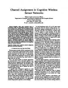
III. CHANNEL SOUNDER EQUIPMENT The channel sounder set-up is displayed in Fig. 1. A Mica2 Motes [5, 9] transceiver is used as transmitter and a spectrum analyzer (ROHDE & SCHWARZ FSH-3) is used as receiver, and both of them are placed just over the ground. Taking into account that the goal of this work is to characterize the near ground wireless channel, but not the effects of the antennas, two λ/4 monopoles placed over two λ/4 x λ/4 ground planes are employed, instead of using the Mica2 whip antennas. Both antennas are connected to the transmitter and to the receiver by a low-losses coaxial cable, and are located far from the hardware to minimize its influence (see Fig. 1). The receiver consists of a laptop, a spectrum analyzer and batteries mounted in a woody trolley with absorber foam to reduce near scatter (see Fig. 1).

Fig 1: Photo of the channel sounder set-up in the ground plain scenario

The receiving antenna is placed at one and a half meter far away from the trolley, whereas the transmitting antenna is one meter far away from the Mica2 transceiver. The transmitter sends a constant carrier of 5 dBm (maximum radiated power) at 868.2972 MHz and the spectrum analyzer is set to this central frequency.

IV. MEASUREMENTS CAMPAIGNS A. Scenarios Three different outdoor environments are characterized in this work: A ground plain area, a university yard and a green park. The first one is a huge ground plain (quasi ideal flat ground) close to the sea without any important close scatter. In this environment propagation can be considered quasi-ideal. The second one is a university yard with dimensions 50m x 35m surrounded by four-story buildings with reinforced cement floors and walls. Here a lot of multipath components contribute at the receiver. Finally, the third of them is a grass green park slightly curved next to a five-story wall. B. Methodology For all scenarios, the same methodology is applied. Several random positions are chosen for the transmitter, and for each of them the trolley is separated from the transmitter until the received signal is 10 dB over the thermal noise (for this spectrum analyzer the measured noise is -95 dBm for a 10 KHz bandwidth). The steps between the receiver positions and the transmitter are: From 0.5 to 3 meters every 0.5 meters, from 3 to 10 meters every 1 meter and then every 2 meters. Centered at each step (defined above), a space averaging at 5 positions separated 10 cm is done, and for all these five positions a 5 times time averaging is also performed (25 snapshots per step). The experiments are conducted several times at each scenario, and for each environment similar results are obtained in different runs. The slow time variance assumption was checked; it was observed that the time variability of the measurements in each position was negligible.

3 V. RESULTS

0.18

L ( d ) = L0 + 10n log10 ( d ) + Xσ

0.14 0.12 0.10 0.08 0.06 0.04 0.02 0.00 -8

-6

-4

-2

 L0 + 10n1 log10 ( d ) + Xσ , d ≤ d r  1 L (d ) =  1 + + 10 log , d > dr L n d X ( ) σ  0 2 10 2  2

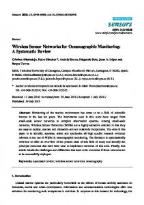
(2) Where in (1) L 0 is the path loss at 1 meter, n is the decay factor, d is the distance expressed in meters, and X σ is a lognormal variable with standard deviation of σ (expressed in dB). In (2) two different slopes are defined before and after a breakpoint dr. For each measured environment these models were applied to each run. It can be clearly observed that a two slopes model fits quite well with the measurements (Fig. 2). Also, the probability distributions of X σ , X σ and X σ have 1

2

been studied. Fig3, 4 and 5 shows the probability density functions of X σ , X σ and X σ . 2

0

2

4

6

8

Xσ(dB)

Fig 3. Probability Distribution Function of X σ (one slope model)

It can be observed that X σ does not follow a Gaussian

X σ 1 and X σ 2 do. An exhaustive

distribution, whereas

(1)

1

0.16

Probability Density Function of Xσ

Fig. 2 shows the results for one run in the first scenario according to the methodology explained above (time averaged received power). It can be seen that the received power fits a straight line using the method of least square errors (logdistance attenuation) when the distance is expressed in dB [15]. The same behaviour is found in the other measurements and scenarios. Therefore, a log-normal path loss model may be considered (the normality is checked below). In addition, the antenna heights are very low (less than λ), and an important part of the Fresnel zone is always obstructed by the ground, so a two-segment least-square fit line may also be used. Then, at each scenario two models are compared, one slope logdistance path loss model and two slopes log-distance path loss model. These models can be denoted by expressions (1) and (2) [10].

measurements campaign would be needed to increase the resolution of these results. The two high peaks of Fig. 3 are due to the mismatch of the one slope model with the measurements. For all the cases under study, all the results were averaged and they are summarised in table I. It is observed that the breakpoint depends on the environment, and that it cannot be calculated as in [15], where it is said that it only depends on the antennas height and the carrier frequency (13 cm for this configuration). The park scenario was slightly curved, which explains that the breakpoint becomes even closer to the transmitter (a bigger Fresnel zone is intercepted by the ground). Comparing both models, it is revealed that a two slopes model leads to a more accurate channel characterisation, and that the standard deviation decreases and its probability density function fits better into a Gaussian. In addition, in this model n 2 tends to 4, which is the expected value for a line of sight situation after the breakpoint. This parameter is crucial for a simulator, because it is going to fix the maximum transmission range of a node. 0.25

-30

Measured

-40

1 slope model 2 slopes model

-50

-60

-70

-80

-90 1

10

Log-distance to the transmitter log(d(m))

Fig 2: Results for the ground plain scenario

Probability Density Function of Xσ1

Received Power (dBm)

-20

0.20

0.15

0.10

0.05

0.00 -2

-1

0

1

X σ 1 (d B )

Fig 4: Probability Distribution Function of X σ1

2

4 TABLE I ADJUSTMENT MODEL PARAMETERS FOR THE THREE SCENARIOS Ground University Symbol Park Plain Yard 1 slope model

0.20

0.15

n σ

3.07 1.83

3.57 3.27

3.69 1.42

dmax (m)

189.5

41.3

52.4

n1 n2 σ1 σ2 Breakpoint (m)

2.35 3.6 0.6 0.42

2.76 4.01 2.98 1.82

2.18 3.95 0.28 0.67

6.2

3.2

0.95

dmax (m)

139.8

32.4

45.7

0.10

2 Slopes Model

Probability Density Function of Xσ2

0.25

0.05

0.00 -1.5

-1.0

-0.5

0.0

0.5

1.0

1.5

Xσ2(dB)

Fig 5: Probability Distribution Function of X σ 2

In table I the maximum averaged radio coverage was calculated for a transmitted power of 5 dBm and a sensitivity of -100 dBm using both models. It is concluded that the two slopes model is more restrictive than the one slope model.

VI. CONCLUSIONS Multiple research papers in the field have presented simulation results for Wireless Sensor Networks. The majority of these works rely on simplistic physical layer assumptions of channel models that can lead to mistaken results. In this paper we present the results of several measurements campaigns that have been performed in order to obtain more accurate and low-computational near ground channel models to feed realistic simulation for the emergent WSN technology. This may contribute to obtain more reliable results and conclusions of protocol performance. Three different scenarios/environments have been characterized and the same methodology has been applied. It has been validated a two slope lognormal channel model at 868 MHz that achieves a more accurate propagation characterization than those of one slope. It also achieves a more accurate propagation characterization than those of one slope, which do not follow a lognormal distribution. Model parameters for WSN propagation are provided. They can be used to adjust ns-2 propagation model for WSN simulation. The two-slope lognormal provides improved accuracy and does not increase computational cost, being suitable for large scale WSN simulations.

ACKNOWLEDGMENT This work has been partially founded by the Economic, Industry, and Innovation Council of the Murcia Region from Spain, under the research project SOLIDMOVIL (2I04SU044) and by Fundacion Seneca under the ARENA Project (00546/PI/04).

REFERENCES [1]

[2]

[3]

[4]

[5] [6]

[7] [8] [9] [10] [11]

[12] [13] [14]

[15]

I. F. Akyildiz, W. Su, Y. Sankarasubramaniam, E. Cayirci. A Survey on Sensor Networks, {IEEE Communications Magazine}, vol. 40, no. 8, pp. 102--116, 2002. Szewczyk, R., Mainwaring, A., Polastre, J., Anderson, J. and Culler, D.: ‘An analysis of a Large Scale Habitat Monitoring Application’, In Proc. ACM SenSys, Baltimore (USA), November 2004. Ganesan, D., Estrin, D., Woo, A., and Culler, D.: ‘Complex Behavior at Scale: An Experimental Study of Low-Power Wireless Sensor Networks’ Technical Report UCLA/CSD-TR 02-0013, Center for Embedded Networked Sensing, University of California, Berkeley, February 2002. Zhou, G., He, T., Krishnamurthy, S., and Stankovic, J.A.: ‘Impact of Radio Irregularity on Wireless Sensor Networks’, In Proc. ACM MobySys, Boston (USA), June 2004. Mica Motes, http://www.xbow.com Kotz, D., Newport, C., Gray, B., Liu, J., Yuan, Y., and Elliott, C.: ’Experimental evaluation of wireless simulation assumptions’. In Proc. of the 7th ACM/IEEE International Symposium on Modeling, Analysis and Simulation of Wireless and Mobile Systems (MSWiM'04), Venice, Italy, October 4-6, 2004. pp. 78-82. Naoumov V., Gross T., ‘Simulation of large ad hoc networks’, MSWiM, San Diego, September 2003 The network simulator ns-2, http://www.isi.edu/nsnam/ns/ Chipcon CC1000, http://www.chipcon.com T. S. Rappaport, Wireless Communications, New York, Prentice Hall, 1996. Sohrabi, K., B. Manriquez, and G. Pottie: ‘Near-ground wideband channel measurements’, Proceedings of the 49th Vehicular Technology Conference. New York: IEEE, 1999, pp. 571-574. J. Zhao and R. Govindan. ‘Understanding Packet Delivery Performance in Dense Wireless Sensor Networks’. ACM SenSys, November 2003. A. Woo, T. Tong, D. Culler: ‘Taming the Underlying Issues for Reliable Multihop Routing in Sensor Networks’. ACM SenSys, November 2003. N. Reijers, G.P. Halkes, K.G..Langendoen: ‘Link Layer in Sensor Networks’. IEEE International Conference on Mobile Ad-hoc and Sensor Systems, Florida (USA), October 2004. H.L. Bertoni, Radio Propagation for Modern Wireless Systems, New Jersey: Prentice Hall, 2000.