Under dc voltage bias, undamped time-dependent oscillations of the current (due to the motion and recycling of electric field domain walls) have been observed ...
Chaos in resonant-tunneling superlattices O. M. Bulashenko† and L. L. Bonilla Universidad Carlos III de Madrid, Escuela Polit´ecnica Superior, Butarque 15, 28911 Legan´es, Spain (February 1, 2008) Spatio-temporal chaos is predicted to occur in n-doped semiconductor superlattices with sequential resonant tunneling as their main charge transport mechanism. Under dc voltage bias, undamped time-dependent oscillations of the current (due to the motion and recycling of electric field domain walls) have been observed in recent experiments. Chaos is the result of forcing this natural oscillation by means of an appropriate external microwave signal.
arXiv:cond-mat/9506030v1 7 Jun 1995
PACS numbers: 73.20.Dx, 73.40.Gk, 47.52.+j, 47.53.+n
al.13 Experimental studies have been carried out by Kahn et al.14 on ultrapure p-Ge, where the NDR is caused by negative differential impurity impact ionization,15 and the transition to a chaotic attractor with loss of spatial coherence has been observed. We consider a set of weakly interacting quantum wells (QWs) characterized by average values of the electric field Ei (t), and the electron density ni (t), with i = 1, . . . , N denoting the QW index. This mean-field-like approach is often justified because the relevant time scale for the oscillations (∼ 0.1 µs) is much larger than those for the tunneling process between adjacent QWs (∼ 1 ns) and the relaxation from excited levels to the ground state within each QW (∼ 1 ps).9 The one-dimensional equations governing the dynamics of the system are the Poisson equation averaged over one SL period l, Amp`ere’s equation for the balance of current density and the voltage bias condition:
Nonlinear oscillations and chaos have been predicted in systems where a predominantly quantum dynamics is corrected by mean-field nonlinear terms due to collective interactions (Hartree)1 or to interactions with classical subsystems having a widely different time scale.2 These phenomena are different from quantum chaos,3 i.e., the behavior of quantum systems whose classical counterpart is chaotic. So far chaotic oscillations have been predicted for systems with few degrees of freedom and experimental evidence is scarce. In this paper we predict chaotic behavior with loss of spatial coherence in a system with many degrees of freedom for which the main transport mechanism is resonant tunneling: a weakly-coupled multiquantum well superlattice (SL). As far as we know these are the first results on chaotic behavior in SLs. In contrast to unbiased triple-well heterostructure,1 our SL is subject to external dc+ac bias, as it was the case with the two-level system of Ref. 2. Very recently time-dependent oscillations of the current on GaAs/AlAs SLs subject to dc voltage bias have been found.4 The oscillations are damped for undoped photoexcited SLs and undamped for doped SLs without photoexcitation.5 For large values of the photoexcitation or the doping, there is stable formation of stationary electric field domains leading to the well-known oscillatory I-V characteristic.6,7,8 According to a discrete drift model,9 the current oscillations are caused by the creation, motion and recycling of domain walls separating two electric field domains.10 This situation is reminiscent of that found in bulk semiconductor devices with negative differential resistance (NDR), where dc voltage bias gives rise to high-field domain dynamics and the wellknown Gunn oscillations.11,12 A significant difference is that the space charge waves are dipoles in the Gunn oscillations and charge monopoles in the SL current oscillations. Another is that the Gunn waves are generated close to the injecting contact whereas the domain walls appear clearly inside the SL.10 Having found a system with a natural oscillation due to traveling-wave motion, it is natural to ask whether harmonic forcing would lead to chaos with spatial structure. The answer is affirmative. This is also the case for the periodically driven Gunn diode studied by Mosekilde et
1 e (Ei − Ei−1 ) = (ni − ND ) l ǫ dEi + eni v(Ei ) = J ǫ dt N X Ei = V (t). l
(1) (2) (3)
i=1
Here ǫ, e, and ND are the average permittivity, the electron charge, and the average doping density, respectively.16 The total current density J(t) is the sum of the displacement current and the electron flux due to sequential resonant tunneling eni v(Ei ). The effective electron velocity v(E) exhibits maxima at the resonant fields for which the adjacent levels of neighboring QWs are aligned,17 as shown in the inset of Fig. 1. The voltage V (t) in (3) is the sum of a dc voltage Vb and an ac microwave signal of relative amplitude A and driving frequency fd : V (t) = Vb {1 + A sin(2πfd t)}. The boundary condition ǫ(E1 −E0 )/(el) = n1 −ND = δ allows for a small negative charge accumulation in the first well, which is taken to be δ ∼ 10−3 × ND . The physical origin of δ is that the n-doped SL is typically sandwiched between two n-doped layers with an excess of electrons, thereby forming a n+ -n-n+ diode.5 Then some charge will be trans1
ferred from the contact to the first QW creating a small dipole field that will cancel the electron flow caused by the different concentration of electrons at each side of the first barrier. To study our equations, it is convenient to render them dimensionless, using the characteristic physical quantities. As the unit of the electric field E = E/E1−2 we adopt the typical electric field strength needed to align the first and the second electron subbands of the nearest QWs E1−2 . The dimensionless velocity v(E) is obtained normalizing v(E) by its value at E = E1−2 , where it has a local maximum due to resonance in tunneling (see inset of Fig. 1). The others dimensionless quantities are defined as follows: the donor concentration ν = elND /ǫE1−2 ; the time τ = t/ttun where ttun = l/v(E1−2 ) is the characteristic tunneling time; the dc bias V = Vb /E1−2 lN ; the ac bias amplitude a = AV; the driving frequency ω = 2πfd ttun . By time-differentiating (3) and using Amp`ere’s law (2), one can express the current density as N ǫ dV e X nj v(Ej ), J(t) = + lN dt N j=1
frequency of the oscillation is mainly determined by the number of QWs the monopole moves across (which increases with N ) and by the average drift velocity.10 Now consider the ac case. We start with a uniform initial field profile and solve the equations for dc bias. After a short transient, the self-sustained oscillations set in and we switch on the ac part of the bias. Our main result is that the competition between the natural oscillation due to monopole dynamics and the forcing gives rise to narrow windows of spatio-temporal chaos for appropriate values of V, a and ω, and that the size and richness of these windows increases with N . Let us fix the ratio between the natural frequency √ f0 and the driving frequency fd at the golden mean ( 5 − 1)/2. To detect and visualize the chaotic regions in parameter space, we need to define a Poincar´e mapping. The current is a good measure of the amplitude (norm) of the solutions which is illustrated by the use of current vs voltage characteristics as bifurcation diagrams.12 Denoting the period of the ac bias Td = 2π/ω, we adopt as Poincar´e mapping (for each value of a) the current at times τm = mTd , m = 0, 1, . . . (after waiting enough time for the transients to have decayed). The result is the bifurcation diagram in Fig.1. Notice the period-doubling sequences that point to the existence of chaos near their accumulation points. There we have computed the largest Lyapunov exponent and found it positive, which confirms chaos within the windows marked by arrows in Fig.1. The chaotic regions are interspersed with locking to periodic and quasiperiodic regimes. Quasiperiodic routes to chaos have been found at the first and last windows marked with arrows in Fig.1. Notice that the period-2 orbits span the widest parameter region from the narrow chaotic band around a ≈ 0.01 up to the next chaotic region at a ≈ 0.09. For a ≥ 0.145 the solution is attracted to the period-1 orbit with the driving frequency fd . More insight into the transition between chaotic and non-chaotic regions of the bifurcation diagram can be obtained by sweeping-down through it, as follows. We set a0 =0.16 (the leftmost value in Fig. 1, where there is period-1 locking) and take an initial field profile {Ei } = V. We now solve the problem (5), compute Jm = J(mTd ) and find out when the solution is periodic within a 10−5 accuracy. At that time, we stop the simulation, depict all Jm correspondent to the period, store the resulting electric field profile, and use it as initial condition for another simulation with a = a0 − ∆a, ∆a = 2 × 10⁻⁴ . By repeating this process, we arrive at chaotic or quasiperiodic regions of a, where the integration is stopped at a much larger time mTd , with m=2000, and only the last 1000 points are depicted, thereby eliminating transients. Fig.1 is the result of such a sweep-down run. The transition points between different regions in the bifurcation diagram are found to be different when a sweep-up run is made, demonstrating thus hysteresis. To illustrate the spatially chaotic nature of the solutions we pick arbitrarily two far-away QWs and depict the simultaneous values of the electric field at them af-
(4)
and after its substitution into (2) we obtain a system of N equations for the electric field profiles: N dEi 1 X v(Ej ) [Ej − Ej−1 + ν] = dτ N j=1
− v(Ei ) [Ei − Ei−1 + ν] + aω cos(ωτ ),
(5)
which we solved numerically by the fourth-order RungeKutta method with the boundary condition E0 = E1 −νδ and initial conditions Ei (0) = V, ∀i. As an example, we consider a GaAs/AlAs SL at T =5 K with N =40, l=13 nm, E1−2 ≈105 V/cm, ND ≈1.15×1017cm−3 , for which undamped time-dependent oscillations of the current were first observed.5 One get ν ≈ 0.1, ttun ≈ 2.7 ns, and we take V=1.2 (corresponding to Vb ≈7.8 V). The main features of our numerical results are as follows. For the dc case (a=0) undamped time-periodic current oscillations of frequency f0 ≈ 9 MHz, (in excellent agreement with the observed value5 ) set in after a transient period. The electric field and charge profiles corresponding to one period of the current oscillation are similar to those found in the undoped case (cf. Figure 9 in Ref. 9). During each period a domain wall (charge monopole) is formed inside the SL. It then moves towards the corresponding contact. Depending on the applied voltage, it may or may not reach the end of the SL before it dissolves and a new monopole is formed starting a new period of the oscillation. Since in a 40-period SL the wall moves only a few QWs, it may be hard to distinguish this monopole recycling from a true spatial oscillation of a single monopole. Simulations of longer SLs (N ≥100), however, clearly show monopole recycling with two monopoles coexisting during some part of one current oscillation period. The 2
3
ter each period of the driving force Td . The resultant attractors for several amplitudes a are presented in Fig. 2. The first example [Fig. 2(a)] shows a chaotic attractor with layered structure and variation in the density of points. The chaotic attractor of Fig. 2(b) has several separate branches almost continuously filled. Finally Fig. 2(c) corresponds to a value of a on the quasiperiodic region. The closed loop with periodic pattern [see Fig. 2(d)] indicates quasiperiodicity: the orbit fills the attractor (torus), never closing on itself. The points in the chaotic attractors cluster with varying density on different regions, which means that they can be characterized by their multifractal dimension Dq (calculated by the method of Ref. 18). We have found that for the particular case of Fig. 2(a), Dq decreases from D−∞ ≈ 1.57 to D+∞ ≈ 0.72, going through the capacity dimension D0 ≈ 1.18. Loss of spatial coherence in the chaotic regime is easily found in long SLs. Density plots for the electron concentration (dark regions mean high electron density) in a 200-period SL with natural frequency ≈ 1.9 MHz are shown in Fig. 3. The density plots show the transition from periodic [Fig. 3(a)] to chaotic domain wall dynamics with loss of spatial coherence [Fig. 3(b)]. Under dc + ac driving with golden mean frequency ratio, nucleation of monopole wavefronts occurs more frequently: in addition to long-living waves travelling over almost the whole SL, there are short-living waves. The two types of waves are distributed chaotically in space and nucleated both at the beginning and deep inside the SL. Detailed calculations show coexistence of up to three monopoles connecting four electric field domains during certain time intervals. We thus have that the loss of spatial coherence is due to chaotic domain-wall dynamics, as seen in Fig. 3(b). In conclusion, spatio-temporal chaos is expected to occur in weakly-coupled semiconductor superlattices (with sequential resonant tunneling as the main transport mechanism) under appropriate dc+ac voltage bias. This prediction should be experimentally testable in currently available n-doped GaAs/AlAs samples forming n+ -n-n+ diodes.5 We thank J. M. Vega and C. Martel for valuable discussions. O. M. B. has been supported by the Ministerio de Educaci´on y Ciencia of Spain. This work has been supported by the DGICYT grant PB92-0248, and by the EC Human Capital and Mobility Programme contract ERBCHRXCT930413.
F. Haake, Quantum signatures of chaos (Springer, Berlin, 1991). 4 S.H. Kwok, T.B. Norris, L.L. Bonilla, J. Gal´ an, J.A. Cuesta, F.C. Mart´ınez, J. Molera, H.T. Grahn, K. Ploog, and R. Merlin, Phys. Rev. B 51, 10171 (1995). 5 J. Kastrup, R. Klann, H.T. Grahn, K. Ploog, L.L. Bonilla, J. Gal´ an, M. Kindelan, M. Moscoso, and R. Merlin, (1994), unpublished. 6 H. T. Grahn, R. J. Haug, W. M¨ uller, and K. Ploog, Phys. Rev. Lett. 67, 1618 (1991). 7 D. Miller and B. Laikhtman, Phys. Rev. B 50, 18426 (1994). 8 F. Prengel, A. Wacker, and E. Sch¨ oll, Phys. Rev. B 50, 1705 (1994). 9 L. L. Bonilla, J. Gal´ an, J. Cuesta, F. C. Mart´ınez, and J. M. Molera, Phys. Rev. B 50, 8644 (1994). 10 L. L. Bonilla, in Nonlinear Dynamics and Pattern Formation in Semiconductors and Devices, edited by F.-J. Niedernostheide (Springer Verlag, Berlin, 1995), Chap.1. 11 M. P. Shaw, V. V. Mitin, E. Sch¨ oll, and H. L. Grubin, The Physics of Instabilities in Solid State Electron Devices (Plenum, New York, 1992). 12 L. L. Bonilla and F. J. Higuera, Physica D 52, 458 (1991); F. J. Higuera and L. L. Bonilla, Physica D 57, 161 (1992); I. R. Cantalapiedra, L. L. Bonilla, M. J. Bergmann, and S. W. Teitsworth, Phys. Rev. B 48, 12278 (1993). 13 E. Mosekilde, R. Feldberg, C. Knudsen, and M. Hindsholm, Phys. Rev. B 41, 2298 (1990); E. Mosekilde, J. S. Thomsen, C. Knudsen, and R. Feldberg, Physica D 66, 143 (1993). 14 A. M. Kahn, D. J. Mar, and R. M. Westervelt, Phys. Rev. Lett. 68, 369 (1992). 15 L. L. Bonilla and S. W. Teitsworth, Physica D 50, 545 (1991). 16 The doping density ND has been incorporated into the equations of Ref. 9, and the hole density has been set equal to zero, as we do not include photoexcitation due to laser illumination in this paper. 17 In our calculations we use the curve v(E ) obtained from the experimental current-voltage characteristics of Ref. 5, as explained in Ref. 4. 18 T. C. Halsey, M. H. Jensen, L. P. Kadanoff, I. Procaccia, and B. I. Shraiman, Phys. Rev. A 33, 1141 (1986).
FIG. 1. Bifurcation diagram of the current at times mTd (for sufficiently large m) versus the driving-force amplitude, for a 40-period SL and the golden-mean ratio between natural and driving frequencies. Windows of chaotic solutions are marked by arrows. Inset: Dimensionless velocity as a function of the electric field. The point indicates the electric-field value corresponding to the dc bias V = 1.2 used in the calculations.
FIG. 2. Electric field values E5 and E36 (at two different QWs of the 40-period SL) measured at times mTd for: (a) a=0.088; (b) a=0.101; (c) a=0.14. (d) is a blow-up of the small region inside the rectangle in (c). 104 successive points have been used to depict each attractor.
†
On leave from Institute of Semiconductor Physics, National Academy of Sciences, Pr Nauki 45, 252650 Kiev, Ukraine. 1 G. Jona-Lasinio, C. Presilla, and F. Capasso, Phys. Rev. Lett. 68, 2269 (1992). 2 L. L. Bonilla and F. Guinea, Phys. Rev. A 45, 7718 (1992).
3
FIG. 3. Density plots for the electron concentration in a 200-period SL for: (a) pure dc bias; and (b) dc + ac bias with a=0.112. x- and y-axes correspond to time (in units of 16 ttun ) and QW index respectively. Darker regions indicate high electron density and mark the location of the domain boundary for each time.
4