Graduate School of Science and Technology, Kobe University, Rokko, Nada, ... Department of Systems Engineering, Faculty of Engineering, Kobe University, ...
Int. 1. Non-Linear Mechanics, Printed in Great Britain.
Vol. 20, No. S/6, pp. 493-506,
1985
0020-7462/85 $3.00 + .OO Pergamon Press Ltd.
CHAOTIC BEHAVIOR IN PIECEWISE-LINEAR SAMPLED-DATA CONTROL SYSTEMS TOSHIMITSU USHIO Graduate School of Science and Technology, Kobe University, Rokko, Nada, Kobe, 657, Japan
and KAZUMASA HIRAI Department of Systems Engineering, Faculty of Engineering, Kobe University, Rokko, Nada, Kobe, 657, Japan Abstract-This paper discusses the suthcient conditions for chaotic behavior in piecewise-linear sampled-data control systems by applying Shiraiwa-Kurata’s theorem. First, it is shown that a discrete-time system with a piecewise-linear element is chaotic if the lower-dimensional system induced from the original system has a snapback repeller. Next, this result is applied to a piecewiselinear sampled-data control system. Finally, the chaotic region for a two-dimensional sampled-data control system with a dead zone element is studied, and two types oftransition from a fixed point to a chaotic attractor are studied by numerical simulation. 1. INTRODUCTION
Non-linear systems which are described by differential or difference equations can have unpredictable, quasi-random nontransient behavior. It is called chaos and has been reported in many scientific fields [l]. In the engineering field, chaos has been studied by Duffing’s equation [2], the Josephson-junction line [3], numerical analysis [4], and so on. Kalman has studied chaos in a one-dimensional sampled-data control system [5]. Recently, the authors have numerically observed chaos in two-dimensional sampled-data control systems and found that the increase of the sampling period implies chaos and crises [6]. A crisis is defined to be a collision between a chaotic attractor and a coexisting unstable fixed point or periodic orbit [7]. Moreover, it has been made clear that any sufficiently large sampling period implies chaos in sampled-data control systems with C?-class non-linear elements satisfying certain conditions [8]. Many sufficient conditions for the existence of chaos have been studied. Li and Yorke [9] have proven that a one-dimensional discrete-time system is chaotic if it has periodic points of period 3, and Marotto [lo] and Shiraiwa and Kurata [l 1 ] have extended Li-Yorke’s theorem to a multi-dimensional discrete-time system. Although their works are very remarkable, it is in practice difficult to apply their theorems to multi-dimensional feedback systems. The reason for the difficulty is that, in order to check whether the system satisfies the conditions of their theorems, the global properties of the system must be clear. Recently, Hata [12] has investigated the existence of chaos in Euler’s finite scheme by applying Marotto’s theorem, and pointed out a way to apply their theorems. His work inspired us to prove the existence of chaos in a non-linear sampled-data control system with a C’class non-linear element [8]. This paper discusses the case where a non-linear element is described by a piecewise-linear function, and it will be shown by using Shiraiwa-Kurata’s theorem that sampled-data control systems satisfying certain conditions are chaotic if the lower-dimensional systems induced from the original systems have snapback repellers. Section 2 treats some basic definitions and previous results. It is shown in Section 3 that a certain piecewise-linear discrete-time control system is chaotic if the lower-dimensional subsystem has a snapback repeller. Section 4 discusses the application of the result obtained in Section 3 to a piecewiselinear sampled-data control system. Section 5 shows a chaotic region for a two-dimensional sampled-data control system with a dead zone element. 2. DEFINITIONS
AND PREVIOUS
RESULTS
In this section, we shall present some definitions and sufficient conditions for the existence of chaos. We consider a discrete-time system of the form x(k + 1) = F(x(k)), 493
k = 0, 1, 2,. . .
(1)
T. USHIO and K. HIRAI
494
where x(k) E R” and F: R” + R” is a piecewise-linear. For a map F: R” -+ R” and any integer k, let Fk be the composition of F with itself k times. A point E is called a periodic point of period p if 2 = Fp(ji) and 2 # Fk(X) for 1 5 k 5 p - 1, and p is called a period. If p = 1, that is, Z = F(X), X is called a fixed point. Let B(x, r) be a closed ball in R” of radius r centered at the point x, and for any set S, let Int S denote the interior of S. DF(x) denotes the Jacobian matrix of F at XE R” if it exists. Let XE R” be a fixed point of (1). The point X is called an expanding fixed point of (1) if there exists a positive number r such that F is differentiable in B(J1,r) and that the absolute values of all eigenvalues of DF(x) are greater than 1 for all x E B(Z, r) [lo]. An expanding fixed point Z is called a snapback repeller if there exist a point x, E B(X, r) and a positive integer M with x, # X and F”(x,) is differentiable, and det DF”(x,) # 0 [lo]. While many definitions of chaos have been proposed [ 131, we shall use the following definition originally proposed by Li and Yorke. Dejnition 1 [9, lo]
It is said that a discrete-time system (1) is chaotic if (1) satisfies the following two conditions. i. There exists a positive number N such that, for each integer p 2 N, (1) has periodic points of period p. ii. There exists an uncountable set S satisfying the following conditions, which is called a scramble set. (a) F(S) = S (b) For any x and y E S with x # y, lim supllFk(x) - Fk(y)ll > 0 k-co
lim infllFk(x) - Fk(y)ll = 0. k-w
(c)
For any x ES and any periodic point y of (l), lim supllFk(x) - Fk(y)ll > 0. k-m
Now we shall state sticient conditions for the existence of chaos. A fixed point X of (1) is said to be a hyperbolic fixed point of (1) if F is differentiable in some neighborhood of T1and no absolute values of eigenvalues of DF(i) are equal to 1. If 2 is a hyperbolic fixed point, a local unstable manifold v=(Z) and a local stable manifold I&(X) are defined respectively as follows. w=(X) = {x E B(X, E); lim Fk(x) = Z} k-m
FQ(X)
=
{xd(X,~);;~
F-klB(X,~)(x)
= X}
where E is a small positive number such that F 1B(X, E) is a diffeomorphism. Theorem 1 (Shiraiwa and Kurata
[ 111) Let Xbe a hyperbolic fixed point of (1). A discrete-time system (1) is chaotic if the following conditions are satisfied. i. The dimension u of a local unstable manifold Wy,(X) is positive. ii. There exist a point X~E W&C) (x0 # X) and a positive integer M such that FM is differentiable at x0 and F”(xo)c fl,&). .. . 111. There exists a u-dimensional disc B” embedded in PI&(X) such that B” is a neighborhood of x0 in w&Z), FM 1B”: B” + R” is an embedding, and FM@“) intersects ~,&) transversally at F”(xo).
Chaotic behavior in piecewise-linear sampled-data control systems
495
Remark. If u is equal to n, Theorem 1 is reduced to Marotto’s theorem, that is, (1) is chaotic if (1) has a snapback repeller. 3. CHAOS
IN DISCRETE-TIME
CONTROL
SYSTEMS
First, we consider the following discrete-time system.
xl@ + 1) = f(x,(k), v4’d, w,(k), . . .f cxz(kN xz(k + 1) = Lxl(k) + Lzx&) + g(xdk),+ 1X2(k), . . . ,a+dW
(2)
k = 0, 1, 2,. . . where xi(k) E R”‘, L1 E Rn2Xn1,L2 E Rn2X”Z,EiE R’ (i = 1, 2,. . . , m + l), and both f: R”‘xR”~ + R”’ and g: R”’ x R”’ -_*R”’ are piecewise-linear functions. Let n = nl + n2 and assume that It1 is not equal to zero. When si = 0 for i = 1,2,. . . , m + 1, (2) reduces to the following system. xl(k + 1) = f*(xi(k)) xz(k + 1) = &xl(k)
+ &x2(k) i- g*(xl(k))
(3) (4)
where f*(xl)
%f(x1,0,0,...,0)
g*(xl) A g(x1,0,0,...,0)*
(5)
For simplicity, (3) and (4) are rewritten as follows. x(k + 1) = F(x(k))
(6)
where
Without loss of generality, it can be assumed that the origin 0 = [O; , Oil’ is a fixed point of (6). In this section, it is assumed that Df*(O,) and Dg*(O,) exist, that the absolute values of all eigenvalues of Df*(O,) are greater than 1, and that those of Dg*(Ol) are less than 1. Then the following lemma holds. Lemma 1 It is assumed that Dg*(xl) exists for any xl such that DJ*(x~) exists. Then (6) is chaotic if the origin Ol is a snapback repeller of (3). Remark. We can easily extend Lemma 1 as follows. If Ol is a snapback repeller of (3), there exist a positive integer M and a point xl, E B(Ol, E) for a sufficiently small positive number E such that f*“(~l,) = Ol. If Dg*(f*‘(xl,)) exists for any integer i, then (6) is chaotic. A proof of Lemma 1 is shown in the Appendix. The following theorem is easily proven by Lemma 1. Theorem 2 Under the assumptions of Lemma 1, if (3) has a snapback repeller, then there exists a positive number E* such that (2) is chaotic for any si satisfying Isi1< E* for i = 1,2,. . . , m + 1. Remark. Theorem 2 is a generalization of Marotto’s perturbation theorem [14] in a sense. Next, we consider an output-feedback control system of the form
y(k) = [Cl
Glx(k)
u(k)= r - f6W) NL”
20 516-K
(7)
496
T. USHIOand K. HIRAI
where Xi(k)E R”‘, x(k) = [x,(k)’ x,(k)‘]‘, y(k) E R”‘, u(k) E R’, Aij E RniX”‘,Bi E R”+‘, Ci E R”“” (i = 1,2), r E R’, and f : R’” ---*R’ is a piecewise-linear function. Now we consider the following lower-dimensional system.
xl& + 1) = Allxl(k) + 4
[r -f(Gxl(W)l.
(8)
Then the following theorem can be proven easily by using Theorem 2. Theorem 3
If (8) has a snapback repeller and the absolute values of all eigenvalues of AZ2 are less than 1, then there exists a positive number Esuch that (7) is chaotic for any Al2 and CZ satisfying II~~zII< s and IIGII < 6. 4. CHAOS IN OUTPUT-FEEDBACK
SAMPLED-DATA
CONTROL
SYSTEMS
In this section, we consider a piecewise-linear sampled-data control system shown in Fig. 1, which is described by n(t) = Ax(t) + &4(t) y(t) = Cx(t)
(9)
u(t) = r - fCv(kT))
kT5
t < (k + l)T,
k = 0, 1, 2,. . .
where x(t)E R”, u(t) E R’, y(t)E R”‘, IE R’, A, B and C are suitable matrices, and T is the sampling period. For simplicity, let us assume that no real part of eigenvalues of A is equal to zero. Then (9) is rewritten in the form of the following discrete-time system. x(k + 1) = eATx(k) + A-‘(eAT
- I)&(k) (10)
y(k) = Cx(k) u(k) = r - fCv(k))
/
where x(k) 2 x(kT), y(k)& y(kT), and u(k) i u(kT). Lemma 2 The non-linear function f:R”’ + R’ of (9) is piecewise-differentiable,
and we assume the following conditions. i. The system (10) has two fixed points Z(l) and Ec2)with X(l) # Zc2),DG(X@)(i = 1,2) exists, and det DG(@) # 0 (i = 1,2) where G(x) = x + A-lB[r
- f(Cx)].
ii. The real part of all eigenvalues of A is positive. Then, there exists a sampling period T* > 0 such that, for any T > Tc, (10) has a snapback repeller, that is, (10) is chaotic. Since the proof of Lemma 2 is identical to that of Theorem 3.1 of [lo], it is omitted.
Fig. 1. A non-linear sampled-data control system.
Chaotic behavior in piecewise-linear sampled-data control systems
497
Without loss of generality, we can define as follows.
where xi(k) E R”‘,Ai E RniX”‘,Bi E R”@‘,and Ci E R”“”(i = 1,2). Let us assume that the real part of all eigenvalues of Al and A2 is positive and negative respectively, and that f’: R’” -+ R’ is piecewise-linear. Then (9) is rewritten as follows.
(11) where, for i = 1 and 2, gi(Xr ,XZ; T, C,) g eAtTXi+ A; ‘(eAiT - Ii)Bi [I - f(Cl~l
+
C2~2~1
and Ii denotes an nixni unit matrix. Letting Cz = 0, (11) becomes the following equations. xi& + 1) = gf(x,(k); T) xz(k + 1) = gl(xi(k),&);
13
where
By applying Theorem 3 to (1 l), we can obtain the following theorem. Theorem 4 If (12a) has a snapback repeller for T = Tf , there exists a positive number E (T’) such that (11) with T= T” is chaotic for any C2 satisfying llC211-c e(P). Lemma 2 and Theorem 4 immediately lead to the following corollary. ~OPOllffP~
1
Let
GI(XI) =
XI + Ai’&
Cr -..f(C~x~)l,
and (12a) has two fixed points Xi’) and Xi2)with jl\‘) # ZP). If Gt : R”*-+ R”*is differentiable at X\r) and Z\‘), and det DG(@) = O(i = 1,2), then there exists a sampling period T* satisfying the following condition. For any I’> T*, there exists a positive number E(T) such that (11) is chaotic for any Ct satisfying jlC$ll -=zE(T). Proof. If the assumptions of Corollary 1 hold, then, by Lemma 2, there exists a sampling period T* such that, for any T > I”L, (12a) has a snapback repeller. Therefore, Corollary 1 is proven by Theorem 4. When /lC21iis s~ciently small, Theorem 4 shows that (11) is chaotic if the lowerdimensional system (12a), whose dimension is equal to the number of unstable eigenvalues of A, has snapback repellers. In the control system (1 l), the dimension n1 of x1 is usually one or two, and if nl = 1, it is comparatively easy to check whether (12a) has snapback repellers or not. Accordingly, Theorem 4 is very useful from a practical point of view. It is a very important problem how to calculate the positive nnmber E of Theorem 4, but there is no general way to do it. Tberefore, we have to calculate Efor each system heuristically.
498
T. USHIO and K. HIRAI
In the next section, the value of E for a two-dimensional sampled-data control system with a dead zone element will be calculated. 5.
CHAOS
IN A TWO-DIMENSIONAL DEAD
SAMPLED-DATA ZONE ELEMENT
CONTROL
SYSTEM
WITH
5.1. Chaotic region This section discusses the existence of chaos in the following two-dimensional data control system with a dead zone element.
y(t) =
wherea > O,az < O,bi~Rl,ci~Rl,xi(t)~R’ described by
f(Y)=
sampled-
(13)
[Cl c214t)
kTStl
0
IYI< I y < -1.
i my+m
A
+ R1 is
(14)
Letting x(k) = x(kT), and xi(k) = xi(kT), (13) and (14) are rewritten as follows. i.
If clxI(k) + c2x2(k) > 1, x(k + 1) = A”x(k) + 6(r + m)
ii. If JcIxl(k) + c,x,(k)l x(k+l)=rlT
< 1, z_,]x(k)+br
(15)
iii. If clxl(k) + c,x,(k) < -1, x(k + 1) = Xx(k) + b(r - m) where dlT
ecllT
- 1)ma; ‘blcl
b62 [(ealT -
‘.‘j&
[ - (eaTT(- 1)ma; ‘b2cl
l)a;‘bl
ealT - 1)ma; ‘blcz e’$ - (eozT - l)mai ‘bzcz
1
(eoZT- l)a;‘b,]‘.
The period-doubling bifurcation set and the Hopf bifurcation set for (15) are obtained by the following equations respectively. ala2(ea1T - l)(eaZT - 1) - m[(e”lT - l)(eaZT + l)azbzcl
+ (ealT + 1)(e02T- l)alblcz]
= 0
ala2(e(a1+(12)T- 1) - m[(ehlT - l)e~ZTazblcl + (eazT - l)e”1Talb2c2] = 0.
(16) (17)
Next, we investigate a chaotic region for (15). For simplicity, it is assumed that the input r is zero. Then (15) can have three fixed poinnts Et’), Zc2)and Zt3), namely, x(1) = -xc3) = - [ala2 - m(a2bIcl + alb2c2)lv1m
xC2)= [O 01’.
aA [ alb2
1
Chaotic behavior in piecewise-linear sampled-data control systems
499
Two fixed points jl(r) and Xt3’exist if the following equation holds. (19) The fixed point P’ always exists. If c2 = 0, then the equation representing the behavior of x1 becomes Cix,(k) + b e”lTxl(k) 5x,(k) - b
xl& + 1) = gl(xl(k)) =
x,(k) > 1
(20)
Ixl(k)l < 1 ,x,(k) < -1
where ii A ealT _ (ealT _ l)ma;‘blcl, 6 = (ealT - l)ma;‘bl. Now, we investigate the conditions under which the fixed point Z\‘) = 0 of (20) corresponding to the fixed point Z(2) of (15) is a snapback repeller. For any point xl in a neighborhood (- 1,l) of the fixed point X’:), dgl(xl)/dxl exists, and is greater than 1. Therefore, if g:(l) < 0, then there exists a point xl,, in (- 1,1) such that gl(xl,) = 0, namely, if the following equation holds, then (20) has a snapback repeller.
6 < 0.
Heal= +
(21)
In the following, let al = 1, u2 = -2, bl = b2 = cl = 1 and m = 2. Then, (21) becomes T>
log(2 +
fi).
(22)
A local stable manifold ~,-,JZ’2)) and a local unstable manifold W;&(2)) of (15) at XC2) become the following.
wf&(2’) = {[O w;&‘2’)
x21’; 1x21< WI} 01’; 1x11< l}.
= {[Xl
The orbits x(l) and x(2) of (15) with the initial condition x(O) = [l
x(1) =
[I ;=
and
01’ become
1*
-eZT+4eT-2 (eeZT - l)(e’ - 1)
x(2) =
Let Q E x(1) and R A x(2). If -eZT + 4eT - 2 < 0, and the point 2 where the line QR intersects the x2-axis belongs to W&(‘)), then the fixed point Z(‘) satisfies Theorem 1, that is, (15) is chaotic. Since 2 becomes eT(emZT - l)(eT - l)-’
Z= [
0
I9
a chaotic region for (15) is obtained by the following equations. T> log(2 + $)
(c21< (eT - l)e-=(l
- ee2=)-l.
(23)
The T - c2 parameter plane for (15) is shown in Fig. 2. From (22), the thick line in T-axis indicates the parameters where (20) has a snapback repeller. From (23), regions 1 and 2 indicate chaotic regions. From (16) and (17), the lines LM and MN indicate the perioddoubling bifurcation set and the Hopfbifurcation set respectively, and regions 2 and 3 are the parameter regions where fixed points E(l) and Xt3)are stable. Accordingly, in region 2, stable fixed points and chaos coexist. Moreover, region 4 is the parameter region where periodic points of period 2 which bifurcate from Z(l) and X13’by period-doubling bifurcations are
T. USHIOand K. HIRAI
500
-2 t-
Fig. 2. The T-c2 parameter plane for (15).
stable. From Fig. 2, it is shown that the existence of a snapback repeller in (20) implies the existence of chaos in (15) if c2 < 0.453. Therefore, we can take the positive number E of Theorem 4 larger than 0.453, and a larger value of E can be taken as the sampling period increases. 5.2. Computer simulation By computer simulation, we shall investigate the transition from a fixed point to chaotic attractors. In the following, c2 is fixed at c2 < 1, and the sampling period T is varied. First, we shall study the case where T increases by crossing the line LM. In this case, periodic points of period 2 appear by period-doubling bifurcations, and if c2 is less than 0.28, then they are unstable, and chaotic attractors appear suddenly when T crosses the line LM. If c2 is less than 1 and larger than 0.28, then they are stable, and as T increases further, finite numbers of the successive period-doubling bifurcations occur, and finally, chaotic attractors appear. Figure 3 shows a typical change of the chaotic attractors near the fixed point X(l) by
3.2'
2.4.
x2
c 1.6'
0s.
L O+ -4.4
-3.6
-2.6
-2
-1.2
-0.4
XI
Fig. 3. A typical change of chaotic attractors when the sampling period increases by crossing the line LM. (c2 =0.2) (a)T= 1.00, (b)T= 1.10, (c)T= 1.11; (d)T= 1.29.
0))
501
3.2.
2.4.
X2 1.6.
0.0.
x2 -0.1
-2.4
-4
-3
-1
1 XI
3
T 5
T.
502
USHIO
and K.
HIRAI
2.4.
0.8.
x2
-0.8.
-2.4.
Fig. 4. Two chaotic attractors near the fixed points jz”) and i(3), (cz = 0.2, T= 1.1.)
the increase of the sampling period. Similar phenomena can be observed near the fixed point Zt3).Chaotic attractors take island shapes when they appear (see Fig. 3(a)). The increase of T reduces the number of islands to half, and a part of chaotic attractors approaches the fixed point jl@)= [0 01’ (see Fig. 3(b)). Figure 4 shows two chaotic attractors near the fixed points jl(‘) and Xc31at c2 = 0.2 and T = 1.1. Finally, these two attractors join at E@),that is, a crisis occurs (see Fig. 3(c)), and the joined attractor looks like an inverted Z as in Fig. 3(d) after the crisis occurs. But, if the value of ca is approximately equal to 1, then crises cannot be observed. Next, we shall study the case where T increases by crossing the line MN. In this case, invariant curves appear around the fixed points Z(l) and Xc3)by Hopf bifurcations. Figure 5 shows a typical transition from an invariant curve to a chaotic attractor. Figure 5(a) shows the invariant curve around the fixed point x-(3). As T increases, wrinkles appear (see Fig. 5(b)). A similar phenomenon has been reported by Curry and Yorke [15]. As T increases further, a part of the attractor becomes fractals [ 161, and approaches the fixed point X@)(see Fig. 5(c)). Similar phenomena can be observed around the fixed point x-(l) . Figure 6 shows two chaotic attractors around the fixed points T1(‘)and Xc3),where parameters T and c2 are equal to the same values of Fig. 5(c). Finally, the attractors join at x-t2) , that is, a crisis occurs (see Fig. 5(d)), and the joined chaotic attractor encircles three fixed points Z(l), Xt2)and Xc3’as shown in Figs. 5(e) and (f). 6. CONCLUSIONS
The existence of chaos in piecewise-linear sampled-data control systems has been studied by applying Shiraiwa-Kurata’s theorem. First, it has been shown that a discrete-time system with a piecewise-linear element is chaotic if the lower-dimensional system has a snapback repeller. Next, this result has been applied to a piecewise-linear sampled-data control system, and the conditions under which the system is chaotic were obtained. These conditions are less strict than those obtained by [S]. Finally, the chaotic region, the period-doubling bifurcation sets and the Hopf bifurcation sets for a two-dimensional sampled-data control system with a dead zone element have been studied. Further, by computer simulation, two types of transition from a fixed point to a chaotic attractor have been observed, and crises have also been observed.
503
e-
-0.:
- 0.88.
x2 -0.t 3.
-0 6I.
-I
0
0.4
0.8
1.2
1.6
XI
-0.
-0. x2 -a
-0.1
x2
-
1.6,
0
0.4
0.8
I
I.2
XI 5WW.
a 1.6
a
504
?-;
(e)
I.2
0.‘
x2
-0.4
- 1.2
I
-2
I
-1.2
I
-0.4
’
XI
I
0.4
I
I.2
’
r;
(f)
.I
0‘
x2
Fig. 5. A typical transition from an invariant curve to a chaotic attractor. (~2 = - 1.0.) (a) T = 0.365; (b) T = 0.38; (c) T = 0.47; (d) T = 0.49; (e) T = 0.53; (f) T = 0.56.
Chaotic behavior in piecewise-linear sampled-data control systems
505
x2
Fig. 6. Two chaotic attractors around the fixed points R(i) and jz’“).(cs = - 1.0, T= 0.47.)
REFERENCES 1. R. H. G. Helleman, Self-generated chaotic behavior in non-linear mechanics. In Fundamental Problems in Statistical Mechanics, Vol. 5, pp. 165-233 (1980). 2. Y. Ueda, Explosion of strange attractors exhibited by DutIing’s equation. Ann. N. Y. Acad. Sci. 357,422-434 (1980). 3. K. Maginu, Spatially homogeneous and inhomogeneous oscillations and chaotic motion in the active Josephson junction line. SIAM, J. appl. Math. 43, 225-243 (1983). 4. M. Yamaguti and S. Ushiki, Chaos in numerical analysis of ordinary differential equations. Physica, 3D, 618-626 (1981). 5. R. E. Kahnan, Nonlinear aspects of sampled-data control systems. Proc. Symp. on Nonlinear Circuit Analysis, Vol. 6, pp. 273-312 (1956). 6. T. Ushio and K. Hirai, Bifurcation and chaos in non-linear sampled-data control systems. IFAC 9th World Congress, Budapest, Hungary, July 2-6 (1984). I. C. Grebogi, E. Otto and J. A. Yorke, Crises, sudden changes in chaotic attractors, and transient chaos. Physica, 7D, 181-200 (1983). 8. T. Ushio and K. Hirai, Chaos in non-linear sampled-data control systems. Int. J. Control, 38,1023-1033 (1983). 9. T. Y. Li and J. A. Yorke, Period three implies chaos. Am. Math. Mon. 82,985-992 (1975). 10. F. R. Marotto, Snapback repellers imply chaos in R”. J. Math. anal. appl. 64, 199-223 (1978). 11. K. Shiraiwa and M. Kurata, A generalization of a theorem of Marotto. Proc. Jap. Acad. 56, Ser. A, 286-289 (1980). 12. M. Hata, Euler’s finite difference scheme and chaos in R”. Proc. Jap. Acad. 58, Ser. A, 178-181 (1982). 13. Y. Oono and M. Osikawa, Chaos in non-linear difference equations-I: Qualitative study of (formal) chaos. Prog. theor. Phys. 64, No. 1, 54-67 (1980). 14. F. R. Marotto, Perturbations of stable and chaotic difference equations. J. Math. anal. appl. 72,716-729 (1979). 15. J. H. Curry and J. A. Yorke, A transition from Hopf bifurcation to chaos: computer experiment with maps on R2. Lecture Notes in Maths. 668, 48-66 (1978).
16. B. B. Mandelbrot, The Fractal Geometry of Nature. W. H. Freeman, San Francisco (1982).
APPENDIX Proof of Lemma 1
In this appendix, we shall prove Lemma 1 by applying Theorem 1. Since the Jacobian matrix DF(0) of F at the origin 0 is
Df*(w
DF(o) =[ Lf
+ Dg*(o,)
0 L2
1’
64.1)
the (global) stable manifold W’(O) of (6) at the origin becomes w”(0) = {[x1
x2
I'; Xl=&,
XER”‘}.
64.2)
506
T. USHIO and K. HIRAI
Letting the subspace E be an ni-dimensional invariant subspaoe of R” associated with the eigenvalues of Df*(O1), the local unstable manifold w;be(O)of (6) at the origin becomes W,(O) = {XER”;
xeE,
II-4 < 4
(A.3)
where E is a suEciently small positive number such that there exists DF(x) for any 11x11 c: E. It is obvious that the dimension of w,(O) is positive. Additionally, by the assumption of Lemma 1, there exists a point xi, E R”’ (xl, # 0,) and a sequence of nr-dimensional compact sets {Dk}g ,, satisfying the following conditions [lo]. i. f*“(~l,) = Oi, xl,uIntDO 11.f*(Dk) = Dk+I iii. f*IDk:Dk -+ Dk+ 1 is differentiable and, for any x, E DE 1Di, detDf*(xi) # 0. (A.4) iv. Oi l Int DM v. lim f*‘(xr,)
= Oi.
&&e other hand, let a function P: R” + R” be a projection, that is, P(x) = xi for any x = [xi xi]‘. Since P(E) = R”‘, it is easily shown by using the condition (v) that there exists X,E l+&(O) satisfying P(x,) = xi,, and from the condition (i), the following equation holds. FM@,) l w”(O)
(A.5)
We define an ni-dimensional disc D” embedded in w=(O) where P(D”) = Do. It is obvious from the condition (i) that D” is a neighborhood of x, in IV&(O). From the condition (ii), for any i = 1, 2,. , M, P(F’(D”)) = Di.
c4.6)
It is also obvious from (A.4) that there exists DF(x) with detDF(x) = 0 for any XE Uf” IF’(D”). Therefore, F”(Du:D” -+ R” is an embedding. Since it is evident that from the condition (iv) and (A.6) that F”(D”) intersects IV(O), we shall prove that the intersection is transversal. In general, there exist independent n-dimensional vectors vr , v2,. . , v,, such that, for any x E F”(D”), there exist scalars ai(i = 1,2,. . . , nl) satisfying the following equation. “I X =
1 &Vi i=1
+ X,
It is assumed that FM@“) does not intersect lV(0) transversally. Then, without loss of generality, vi is parallel to IV(O), that is, P(Vi) = 01.
(‘4.7)
From (A.7), n, vectors P(vi), P(v& . . . , P(v,,) are linearly dependent, which implies that P(F”(D”)) is not an nldimensional disc. Therefore, from (A.6), DM is not an ni-dimensional disc, which is a contradiction. From these considerations, Lemma 1 can be proven by applying Theorem 1.