Chaotic Dynamics of MLC circuit using MATLAB-SIMULINK Model. Introduction. In this study, we wish to present a detailed numerical investigation of the chaotic ...
Chaotic Dynamics of MLC circuit using MATLAB-SIMULINK Model Introduction In this study, we wish to present a detailed numerical investigation of the chaotic dynamics of the very simple nonlinear dissipative two dimensional non-autonomous electronic circuit, namely the Murali-Lakshmanan-Chua (MLC) circuit. We obtain the phase portrait of the chaotic circuit using the MATLAB-SIMULINK model of the circuit and also by PSIM circuit simulation. In this circuit, a typical period-doubling sequence leading to chaotic motion is found to occur when the amplitude of the external periodic force is varied. We will illustrate in the following how ordered and chaotic motions occur using both MATLAB-SIMULINK model and PSIM circuit simulation. .
Realization of the Circuit The circuit originally introduced by Murali, Lakshmanan and Chua (MLC) is a simple nonautonomous circuit and can be realized as shown in Fig. 1.1. It contains a voltage-
R
L iL
+
iC + C
f(t) RS
v _
NR
Figure 1.1: Circuit realization of the MLC circuit. Here N R is the Chua’s diode. controlled nonlinear resistor (NR ) described by the relation iN = g(v), which in this case is a Chua’s diode [146]. Here C is capacitor, L is an inductor, R is a linear resistor, while R s is a current sensing resistor and f (t)(=f sinΩt) is the external periodic forcing. By applying Kirchoff’s laws to this circuit, the governing equations for the voltage v across the capacitor C and the current iL through the inductor L are represented by the following set of two first order coupled non-autonomous differential equations:
C (dv/dt) = iL – g(v)
(1.1a)
L (d iL /dt) = R iL – Rs iL – v + f sin(Ωt)
(1.1b)
Where, g(v) = Gb v + 0.5(Ga − Gb )[|v + Bp | − |v − Bp |]. (1.1c) In Eq. (1.1c), Bp is the breakpoint voltage of Chua’s diode, f is the amplitude and Ω is the angular frequency of the external periodic signal. The experimental realization of the Chua’s diode is well described by Kennedy . The behavior of the above circuit depends on five control parameters, namely the inductance L, the capacitance C , the linear resistance R, the amplitude f and the frequency ν(=Ω/2π) of the external periodic signal, besides the parameters associated with Chua’s diode (which we usually fix at definite values). The values of the linear circuit elements are fixed as R=1340 Ω, Rs =20 Ω,L=18 mH, C =10 nF and the parameters of the Chua’s diode are chosen as Ga = −0.76 mS,Gb = −0.41 mS and Bp =1.0 V. In their original work, Murali et al. have studied the dynamics of the circuit given by Eq. (3.1), by fixing the frequency, ν(=Ω/2π), at 8.89 kHz andvarying the amplitude f in the range (0.05 V, 0.7 V). In this parametric region considered the circuit exhibits several interesting dynamical phenomena including period-doubling bifurcations, chaos and periodic windows. Further it will be quite valuable from nonlinear dynamics point of view to construct a phase portrait for an extended and detailed study.
-K-
Gb*V)
Gb |u| 1
Add
Abs
Add3
Constant -KAdd2
Gain C (dv / dt )
-K-
|u| 1
Add1
Add4
Abs1
(dv /dt )
1/C
1 s
v oltage
integrator 1
Constant1
Out1
-1
XY Graph
-V
Scope1
-V -K-
-(Rs + R)
Gain3
L (diL/dt)
Add5
-K1/L
(diL/dt)
1 s
current
Integrator1
f sin(w*t)
Sine Wave
Figure 1.2: MATLAB-SIMULINK model of the MLC circuit
2 Out2
Figure 1.3: PSIM model of the MLC circuit
-4
-6
x 10
Current
-6.5 -7 -7.5 -8 -8.5 -9 0.01
0.011
0.012
0.013
0.014
0.015
0.016
0.017
0.018
0.019
0.02
0.016
0.017
0.018
0.019
0.02
Time 1.25 1.2
1.1 1.05 1 0.95 0.9 0.85 0.01
0.011
0.012
0.013
0.014
0.015
Time
(a) -4
-6
x 10
-6.5
-7
Current
Voltage
1.15
-7.5
-8
-8.5
-9 0.85
0.9
0.95
1
1.05
1.1
1.15
1.2
1.25
Voltage (b)
Figure 1.4: (a)time series plot of period 1 limit cycle (b) phase portrait of period 1 limit cycle
1.4 1.3
Current
1.2 1.1 1 0.9 0.8 0.7 0.01
0.011
0.012
0.013
0.014
0.015
0.016
0.017
0.018
0.019
0.02
0.016
0.017
0.018
0.019
0.02
Time -4
-4
x 10
-6 -7 -8 -9 -10 0.01
0.011
0.012
0.013
0.014
0.015
Time
(a) -4
-4
x 10
-5
-6
Current
Voltage
-5
-7
-8
-9
-10
0.7
0.8
0.9
1
1.1
1.2
1.3
1.4
Voltage (b) Figure 1.5: (a)time series plot of period 2 limit cycle (b) phase portrait of period 2 limit cycle
-4
-2
x 10
-3
Current
-4 -5 -6 -7 -8 -9 -10 0.01
0.011
0.012
0.013
0.014
0.015
0.016
0.017
0.018
0.019
0.02
0.016
0.017
0.018
0.019
0.02
Time 1.4
1
0.8
0.6
0.4 0.01
0.011
0.012
0.013
0.014
0.015
Time
(a) -4
-2
x 10
-3 -4
Current
Voltage
1.2
-5 -6 -7 -8 -9 -10 0.4
0.5
0.6
0.7
0.8
0.9
1
1.1
1.2
1.3
1.4
Voltage (b)
Figure 1.6: (a)time series plot of period 4 limit cycle (b) phase portrait of period 4 limit cycle
-4
-2
x 10
-3
Current
-4 -5 -6 -7 -8 -9 -10 0.01
0.011
0.012
0.013
0.014
0.015
0.016
0.017
0.018
0.019
0.02
0.016
0.017
0.018
0.019
0.02
Time 1.6 1.4
1 0.8 0.6 0.4 0.2 0.01
0.011
0.012
0.013
0.014
0.015
Time
(a)
-4
-2
x 10
-3 -4
Current
Voltage
1.2
-5 -6 -7 -8 -9 -10 0.2
0.4
0.6
0.8
1
1.2
1.4
Voltage (b) Figure 1.7: (a)time series plot of one band chaos (b) phase portrait of one band chaos
1.6
-3
1.5
x 10
Current
1 0.5 0 -0.5 -1 -1.5 0.01
0.011
0.012
0.013
0.014
0.015
0.016
0.017
0.018
0.019
0.02
0.016
0.017
0.018
0.019
0.02
Time 1.5
0 -0.5 -1 -1.5 0.01
0.011
0.012
0.013
0.014
0.015
Time
(a) -3
1.5
x 10
1
0.5
Current
Voltage
1 0.5
0
-0.5
-1
-1.5 -1.5
-1
-0.5
0
0.5
1
Voltage (b) Figure 1.8: (a) time series plot of two band chaos (b) Phase portrait of period two band chaos
1.5
-3
1.5
x 10
Current
1 0.5 0 -0.5 -1 -1.5 0.01
0.011
0.012
0.013
0.014
0.015
0.016
0.017
0.018
0.019
0.02
0.016
0.017
0.018
0.019
0.02
Time 2 1.5
0 -0.5 -1 -1.5 -2 0.01
0.011
0.012
0.013
0.014
0.015
Time
(a) -3
1.5
x 10
1
0.5
Current
Voltage
1 0.5
0
-0.5
-1
-1.5 -2
-1.5
-1
-0.5
0
0.5
1
1.5
Voltage (b) Figure 1.9: (a)time series plot of period 3 limit cycle (b) phase portrait of period 3 limit cycle
2
-3
1.5
x 10
Current
1 0.5 0 -0.5 -1 -1.5 0.01
0.011
0.012
0.013
0.014
0.015
0.016
0.017
0.018
0.019
0.02
0.016
0.017
0.018
0.019
0.02
Time 1.5
0.5 0 -0.5 -1 -1.5 0.01
0.011
0.012
0.013
0.014
0.015
Time
(a)
-3
1.5
x 10
1
0.5
Current
Voltage
1
0
-0.5
-1
-1.5 -1.5
-1
-0.5
0
0.5
1
1.5
Voltage (b) Figure 1.10: (a)time series plot of period 1 boundary (b) Phase portrait of period 1 boundary
(a)
(b) Figure 1.11: (a) Time series plot of voltage and current for one band chaos in PSIM (b) Phase portrait for one band chaos
(a)
(b) Figure 1.12: (a) Time series plot of voltage and current for two band chaos in PSIM (b) Phase portrait for two band chaos
The dynamics of the MLC circuit is as shown in the above figures. Figures 1.4 to 1.9 show the dynamics of the MLC circuit solved numerically using MATLAB-SIMULINK model shown in figure (1.2). The SIMULINK model is created such that the MLC circuit equation is modeled in terms of mathematical blocks and the output is either obtained through an XY graphical block or by means of a SCOPE block. The circuit equation is solved for the Voltage across the capacitor and current across the inductor. The output thus results can also be stored in MATLAB workspace and the results thus obtained can then be plotted using MATLAB commands or scripts in the command window or through an m file. Now let us analyze the dynamics of the MLC circuit. As stated earlier, the amplitude of the external force acts as the control parameter and the frequency of the force is kept as a constant. The dynamics of the system depends upon the amplitude and frequency of the forcing term. By varying the amplitude of the force the system bifurcates to chaos through the period doubling sequences. When the amplitude of the force is kept at f=0.05 V, the system shows steady state oscillations and hence exhibits a stable limit cycle in its dynamics. Figure 3.4 (a) shows the time series plot of the Voltage across capacitor and current in the inductor. Figure 3.4 (b) shows the phase portrait of the system in the V-I phase plane. The phase trajectory is a stable limit cycle. When the amplitude of the force is f=0.075 the dynamics is a period two limit cycle. The time series plot and the phase portrait of the period two limit-cycle are shown in figures 1.5 (a) and (b) respectively. When the amplitude of the force is increased to f=0.0875, the system exhibits a period-4 limit cycle oscillation. The corresponding time series plots and phase portraits are shown in figures 1.6 (a) & (b). Further increase in amplitude of the force leads to further doubling of the periods and the system becomes chaotic for the force value f=0.1 V. The time series plot of the voltage and current is shown in figure 1.7 (a). The phase portrait shows that the trajectories never overlap each other and also that it is bounded to a particular region of phase space. This phenomenon of unpredictability of the dynamics of the system in a bounded region of space is called chaos. The time series plot and the phase portrait of one band chaos is shown in figure 1.7 (a) & (b). With further increase in the amplitude of the force, two-band chaos is observed in
the dynamics. The corresponding time series plot and phase portrait are as shown in figures 1.8 (a) & (b). Chaos does not have a periodic pattern but it has a fractional order dimension associated with it. Hence the dynamics of the system bifurcates from periodic motion to bounded aperiodic motion. This kind of sudden qualitative changes in the dynamics of the system is called as bifurcation. Period doubling route is one such route to chaos, which is observed in the MLC circuit for the particular set of circuit parameters for this current study. Further the dynamics of the system in the chaotic region have sensitive dependence on initial conditions i.e. when the system is evaluated to chaos for two different initial conditions the dynamics dynamics differ entirely. The chaos presented in this thesis is not characterized because nonlinear dynamical systems are expressed by nonlinear differential equations whose analytical solutions are highly complicated. Further no general methods are available for solving a set of nonlinear differential equations. Hence these nonlinear equations are often solved numerically and the characterizations are done based on the numerical data thus obtained. With further increase in the force value the system exhibits a period-3 limit cycle motion for f=0.245 V. The time series and phase portraits are shown in figure 1.9. The system approaches the boundary when the force f=0.63 V as shown in figure 1.10. The chaotic dynamics of the MLC circuit is further confirmed through PSIM simulation of the circuit shown in Fig. 1.3. The one-band and double band chaotic attractors exhibited by the circuit for two different values of the f=0.06 V and f=0.135 V are shown in Fig. 1.11 and Fig.1.12 respectively.
In this study, the chaotic dynamics of a simple nonlinear electronic circuit namely the MuraliLakshmanan-Chua (MLC) is studied through MATLAB-SIMULINK modeling of the normalized circuit equations. The results are confirmed by PSIM simulation of the circuit.