OUTBREAK-CRASH DYNAMICS AND CHAOTIC

OUTBREAK-CRASH DYNAMICS AND CHAOTIC INTERACTIONS OF COMPETITION, PREDATION, PROLIFICACY IN SPECIALIST FOOD WEBS BRIAN BOCKELMAN, BO DENG, ELIZABETH GREEN, GWENDOLEN HINES, LESLIE LIPPITT, AND JASON SHERMAN Abstract. A basic food web of 4 species is considered, of which there is a bottom prey X, two predators Y, Z on X, and a super predator W only on Y . The study concerns with classifying long-term trophic dynamics and shortterm population outbreaks/crashes in terms of species characteristics in competitiveness, predatory efficiency, and reproductive prolificacy relative to the web. It also concerns with the interplay between mathematics and ecology in developing a set of holistic principles complementary to the technical method of singular orbit analysis which we use. The main finding is that enhancement in Z’s reproductive prolificity alone can lead to long-term trophic destabilization from equilibrium to cycle to chaos, and short-term outbreak/crash phenomena in the web.

1. Introduction Competition, predation, and proliferation are fundamental forces that drive ecological systems. Understanding how these forces come to shape basic food webs that contain some minimum numbers of species is no doubt a necessary step to unravel ecocomplexity. When isolated, each factor is known to play a unique role in population dynamics. With one predator and one prey, Rosenzweig’s Enrichment Paradox ([25]) leads to population destabilization. With one prey and two predator, the coexisting states are prescribed by the Competition Exclusion Principle ([14]). With nonoverlapping population dynamics, enhancement in prolificity leads to the phenomenon of period-doubling to chaos ([18]). By some much less understood mechanisms chaotic dynamics occurs in 3-trophic food chains and polyphagous predator-prey webs ([13, 11]). The purpose of this paper is to give a comprehensive and unified treatment to the interplay of these factors in the context of a basic food web model. This is a theoretical attempt. Selection of generic models is critical to the plausibility of the result. Although ecological systems follow few laws and rules that are subject to first principle derivation, there are two well-accepted modelling principles on which our models will be solely based. Like others before us, we will use Verhulst’s logistic growth principle ([28, 17, 29]) for the bottom prey, denoted by X in density, by assuming that X’s per-capita birth rate is constant b0 , and its per-capita death rate is quasi linear: d + d0 X with d, d0 > 0, which is likely the result of environmental limitations, interspecific competition, to name just two This work was funded in part by an NSF REU grant, #0139499, for the summer of 2002. B. Deng, G. Hines were the REU advisors. B. Bockelman, E. Green, L. Lippitt, and J. Sherman were the REU participants. 1

2

B.BOCKELMAN, B.DENG, E.GREEN, G.HINES, L.LIPPITT, & J.SHERMAN

situations. The rate balance equation gives rise to prey’s per-capita growth rate equation: X1 dX dt = b0 − d − d0 X. With the maximum per-capital growth rate r = b0 − d and the carrying capacity K = r/d0 , we have the standard logistic model dX X dt = rX(1 − K ) for the prey. The second modelling principle is based on Holling’s seminal work on species predation ([12]). In his original set up, let T be a given period of time, let Y be the population density of a predator of the prey X, and let XT be the captured prey unit per unit predator during the T period of time. Holling identified two important factors intrinsic to most predations: predator’s handling time Th for capturing, killing, consuming, and digesting one unit prey; and the discovery probability rate a which is the product of the search rate s and the probability A of finding a prey. Then, the following simple relations must hold: the time left for searching T − Th XT , and the balance equation XT = a × (T − Th XT ) × X. Solving the last equation gives rise to XT aX aT X and = , XT = 1 + aTh X T 1 + aTh X with the last being the per-capita predation rate for the predator. Imposing further assumptions on Th and a lead to more specific forms. Assuming Th = 0 results in Holling Type-I predation form aX. This zero handling time assumption is not completely unrealistic. It can be used as a good approximation for, e.g., filter feeders ([24]) as well as parasitoid predation. Assuming a constant discovery rate a results in the most common form of Holling Type-II. Assuming a density dependent discovery rate a = aX n , n > 0 results in the Holling Type-III form, which, e.g., was used for birds-insects predation ([16]). In this paper, we will only use the Holling Type-II form, the most common form of the three, in the following equivalent format aX pX 1 1 = with p = , H= . 1 + aTh X H +X Th aTh Here p represents the saturation (maximum) predation rate when X is abundant (X → ∞), and H the half-saturation density which when X = H the predation is half the saturation rate p. Hence, the simplest predator-prey web model based on these two modelling principle is the following equation µ ¶  X pX dX   = rX 1 − − Y dt K H +X   dY = bpX Y − dY , dt H +X bpX Y is the predator’s birth rate with b being the birth-to-consumption where H+X ratio. Except for the prey X, we will only assume constant per-capita death rates for all predators, instead of Verhulst’s logistic for a reason to be explained later. The long term behaviors of this model are well-understood (see [25, 18]). It can either have a global stable equilibrium or a global stable limit cycle. The Enrichment Paradox states that increasing prey’s carrying capacity K can drive the system from a steady equilibrium state to a limit cycle state. We will call Y a weak predator if the XY asymptotic state is the coexisting equilibrium and an efficient one if the asymptotic state is the limiting cycle.

SPECIALIST FOOD WEBS

3

A basic food web with two predators competing for the same prey but otherwise free of other forms of competition can then be modelled as follows: µ ¶  X p2 X p1 X dX   = rX 1 − Y − Z −   dt K H + X H  1 2+X  dY b1 p 1 X = Y − d1 Y  dt H1 + X    dZ b2 p 2 X   = Z − d2 Z. dt H2 + X In this case, predation is an indirect form of competition, and Holling’s functional forms play the dual roles of both predation and competition. A fair amount is known about this system but by no means complete. Competitor Z is said to be competitive if the XY -attractor (either the stable equilibrium state or the stable limit cycle of the XY -predator-prey system with Z = 0) is unstable with respect to the full XY Z-web. Z is said to be dominant if its XZ-attractor is globally attracting for the XY Z-web. Extend similar definitions to Y . Then the following three alternatives are known so far: (i) If both Y and Z are weak predators, then either Y or Z is dominant and the other must die out; (ii) If both are competitive with at least one being efficient, then they will coexist, not in the form of a steady state but only known in the form of a limit cycle, see [14, 30, 15]. These results are referred to as the Competition Exclusion Principle. A basic tritrophic food chain model takes the following form due to RosenzweigMacArthur ([26]) µ ¶  X p1 X dX   = rX 1 − Y −   K H1 + X   dt dY b1 p 1 X p3 Y = Y − d1 Y − W  dt H + X H 1 3+Y    b p Y dW 3 3   = W − d3 W , dt H3 + Y with the addition of a top-predator W above Y . Though not completely understood, substantial progress has been made recently ([5, 6, 7, 8]). The following dynamics are known to exist. (i) If Y is a weak predator, then either a coexisting stable steady state or a coexisting limit cycle is possible ([20]). The limit cycle is referred to as X-slow with less variation in X than Y and W . (ii) If Y is efficient, (i) may still apply. In addition, it is also possible to have a so-called XY -fast limit cycle with less variation in W than X and Y . More distinctively, when both Y and W are efficient, it is possible to have 4 different types of chaotic attractors ([5, 6, 7, 8]) and extremely complex bifurcations from one type to another. We consider in this paper a web consisting of an XY W -chain and a mid-level competing predator Z which (1) competes with Y for the same prey X according to Holling Type-II predation, (2) does not engage in any other form of competition with Y , (3) is not a prey of W . It can also be viewed as a competing web XY Z with the addition of the top-predator W to Y . It contains the minimum number of species with which we can study the combined effects of predation and competition.

4


Such a system is modelled by equations below:  µ ¶ dX X p2 X p1 X   = rX 1 − Y − Z −    dt K H + X H 1 2+X   dY  b1 p 1 X p3 Y   = Y − d1 Y − W dt H + X H 1 3+Y (1) dZ b2 p 2 X   = Z − d2 Z    dt H 2+X   b3 p 3 Y  dW   = W − d3 W dt H3 + Y

Appendix A gives a formal and generalized treatment to the concepts of chain, web, weak predation, and competitiveness in terms of system dynamics. The relative competitiveness between Y and Z is determined by their predation characteristics on X in terms of weak and efficient predation assumption. Another important factor determining patterns of their interactions is the ratio of their maximum per-capita growth rates. We refer to the ratio as the prolificacy parameter. For example, the X-to-Y ratio is the XY -prolificacy. This leads to a basic assumption we will adopt for this paper. That is, the chain prolificacy diversification assumption for all predator-prey chains regardless of length: in the XY Z-web the per-capita maximum reproductive rate for X is much greater than those of Y, Z, and along the XY W -chain the per-capita maximum reproductive rates for X, Y, W range from high, moderate, to low. In contrast, there should not be an obvious rate preference for the competing Y, Z. However, if the prolificity of Z is greater than that of Y , then Z should be viewed as becoming more competitive against Y . The main question we are interested in can be posted from two different angles. From a view point of the XY W chain, we ask how its dynamics are affected by including a competing predator Z at the mid-lateral level? Rephrasing the same question from an XY Z web perspective, how do web dynamics change when a top-predator W is introduced? What roles do efficiency, competitiveness, and prolificacy play in the full web dynamics? We will exam in this paper a simpler case when both Y and Z are weak competitors in the XY Z-web for which either Y or Z must die out according to the Competition Exclusion Principle. By imposing W on Y , we expect that the competitive edge of Z is enhanced. Therefore, if Y is not XY Z-competitive, it should remain so and Z will drive out the 2 species Y W chain with the XZ equilibrium remaining. However, if Z is not XY Z-competitive (i.e., it must die out in the XY Z environment since both Y and Z are weak), then under what conditions does Z become XY ZW -competitive, and in what dynamical forms can all species coexist? Since Y is weak, the XY W -chain dynamics can only be steady state or an X-slow limit cycle. Can a weak and XY Z-noncompetitive predator Z break in and survive in the expanded XY ZW community? If yes, could the coexistence state be an equilibrium, which the Competition Exclusion Principle prohibits for the XY Z web? Must it be a limit cycle? Would it permit structures more complex than steady states and limit cycles? Concerning shortterm cyclic dynamics, can it have periods of outbreaks and crashes? How low can the populations crash to? Some main findings are summarized as follows: (a) Top-predation on a single predator in an exclusionary competing web always creates coexisting space for the other predator to be competitive; (b) Top-predatory efficiency and the competitorto-midprey prolificacy enhancement destabilize coexisting equilibrium state into


5

cyclic and chaotic states; (c) Outbreak/crash dynamics are the result of prolificity diversification between week competitors or prolificity diversification between efficient predator and prey. More specifically, (1) If all the predators Y, Z, W are respectively weak, the full system can have an attracting XY ZW equilibrium state if the ZY -prolificacy, ²1 , is small, or an attracting XY ZW limit cycle if ²1 is moderate, or a chaotic attractor if ²1 is large. All these structures are critically dependent of the presence of W . Without it, the dynamics is reduced to the XY W -equilibrium with Z extinct. (2) If Y, Z are weak but W efficient, the full system for small ²1 can have two coexisting XY ZW attractors, one is an equilibrium state, the other a limit cycle, each has its own basin of attraction. (3) For the same predator profiles as (2) above, the full system undergoes a sequence of bifurcations in XY ZW attractors with increasing ²1 : from steady state to limit cycle and to chaotic attractor. The type of chaotic attractors in this case is significantly different from the case of (1) in that it has a greater dynamical variability. The principle of predation inclusion and the route of prolificity enhancement to chaos are unique. They do not have lower dimensional analogues in systems of predator-prey, prey-predator-superpredator, and prey-predators/competitors. The principle of prolificacy outbreak/crash is ubiquitous for all system. Long-term dynamics in terms of equilibrium, limit cycle, chaos, and short-term phenomena in terms of cyclic outbreaks, crashes are recurrent throughout all trophic levels when viewed according to our classification scheme. Thus we argue that all these newly discovered principles should become part of our understanding on population dynamics side by side with other well-known principles such as the Enrichment Paradox, the Competition Exclusion Principle, to form a basis for practical prediction. For example, chaos is invariably linked to predation, competition, and prolificacy enhancement, whereas equilibrium state is strongly associated with weakness in all. Also, population outbreaks and crashes are strongly linked to diverging growth rates. To our best knowledge dynamics of combined chain predation and web competition have not been systematically analyzed in the literature. There are a few understandable reasons. First, systems of dimensions higher than 3 are formidable mathematically, and our XY Z, XY W, XY ZW equations are no exceptions. Second, the full XY ZW system contains 14 parameters, which can become unmanageable if an effective classification scheme is not in place. Because of the lack of such a scheme or as a result of it, we did not have a mathematically concise, ecologically meaningful language to formulate questions or answers. We believe we have succeeded in all these aspects. We developed a minimum number of dynamically defined ecological concepts to classify most if not all dynamical behaviors of the models. These concepts are: weak and efficient predation, competitive and noncompetitive competition, trophic prolificacy for growth. We will demonstrate how these concepts are used to frame trophic interactions and partition the 14 parameter space accordingly. We will carry out our analysis not only mathematically, but more importantly, we will do so by developing a set of equivalent, holistic, practicable principles and rules and using them complementarily to the mathematical

6


analysis. The effectiveness of this approach should become more apparent as more non-aggregatable species are incorporated into a larger web. The paper is organized as follows. In Sec.2 we will scale the model to a nondimensional system for which the prolificacy parameters of all species against Y become exactly the time scales for the dimensionless system. We will summarize some important results in terms of numerical simulations in Sec.3. The remaining sections are more analytical. We will derive in these sections the main results both mathematically and holistically. More specifically, Sec.4 gives an introduction to the methodology of singular orbit analysis, a survey over other methods, and a catalog of mathematically-based ecological principles that will be used later. Sec.5 and Sec.6 summarize some important known results for the competing XY Z-web and the XY W -chain that will not only provide a platform to build the full XY ZW web results but also contrast dynamical behaviors of the full system against its parts. Sec.7 is devoted to classify, analyze, interpret the main results for the full system. Last we will end the paper with a discussion on the conclusions and future directions in Sec.8. 2. Weak, Competitive Predators and Chain Prolificacy As a necessary first step of mathematical analysis, we non-dimensionalize Eq.(1) so that the scaled system contains a minimum number of parameters for simpler manipulation, for uncovering equivalent dynamical behaviors with changes in different dimensional parameters. Using the same scaling ideas of [5] and the following specific substitutions for variables and parameters Y Z W X , z= , w= t → b1 p1 t, x = , y = K Y0 Z0 W0 rK b1 p 1 Y 0 rK , Z0 = , W0 = Y0 = p1 p2 p3 b2 p 2 b3 p 3 b1 p 1 , ²1 = , ²2 = ζ= (2) r b3 p 3 b1 p 1 H2 H3 H1 , β2 = , β3 = β1 = K K Y0 d2 d3 d1 , δ2 = , δ3 = , δ1 = b1 p 1 b2 p 2 b3 p 3 Eq.(1) is changed to this dimensionless form:  µ ¶ dx y z   =x 1−x− − := xf (x, y, z)  ζ   dt β1 + x β2¶+ x  µ  dy  w x   =y − − δ1 := yg(x, y, w)  dt β + x β 3+ µ1 ¶y (3) x dz   = ²1 z − δ2 := zh(x)    dt β  ¶ µ2+x  dw  y   = ²2 w − δ3 := wk(y)  dt β3 + y The choice of these parameters can be explained as follows. The prey density X is scaled against its carrying capacity K, leaving x a dimensionless scalar. The predator is scaled against Y0 , which can be viewed as the predation carrying capacity of the predator. The choice of Y0 is motivated by the relation p1 Y0 = rK, i.e., the rate of capture by Y0 , p1 Y0 , is equal to the capacity growth of the prey, rK. The scaling, y = YY0 gives y a scalar dimension. The scaling of the competitor Z is


7

Table 1. Trophic Characteristic in Reproductive Rate Ratios

Food Chains plant-herbivore-carnivore plankton-zooplankton-fish resource-host-parasitoid tree-insect-bird prey-predator-virous ...

Max. Reproductive Rate Ratios b3 p 3 b1 p 1 ²2 = ζ= r b1 p 1 small (¿ 1) moderate or small small small small small to large large small – large ... ...

done with a similar motivation. The top-predator is scaled against it’s predation carrying capacity, W0 , at which p3 W0 = b1 p1 Y0 with b1 p1 the maximum growth rate and Y0 the Y -predation capacity. The remaining parameters need to be explained a bit more as well. Parameters β1 , β2 , and β3 are the ratios between the semi-saturation constant of the respective predator versus the carrying capacity of the respective prey. They are dimensionless semi-saturation constants in the scaled system (3). Because a decent predator is expected to reach half of its maximum predation rate before its prey reaches its capacity, nature provides us with a reasonable interval: 0 < βi < 1, which we will use for this paper unless said otherwise. The parameters δ1 , δ2 , and δ3 are relative death rates, each is the ratio of a respective predator’s death rate to its maximum birth rate. As a necessary condition for species survival, the predator’s death rate must less than its maximum reproductive rate. Therefore we make a default assumption that 0 < δi < 1 for nontriviality. The remaining parameters, 1/ζ, ²1 , ²2 , are relative maximum growth rates of X, Z, W to Y , i.e., the XY -prolificacy, ZY -prolificacy, and the W Y -prolificacy respectively. By the theory of allometry ([2, 3]), these ratios correlate reciprocally well with the 4th roots of the ratios of X, Z, W ’s body masses to that of Y ’s. Thus they may be of order 1 when predator’s and prey’s body masses are comparable or of smaller order if, as in plankton-zooplankton-fish, and most plant-herbivorecarnivore chains, the body masses are progressively becoming heavier in magnitude so that ζ and ²2 are small parameters. In any case, a given web will find its corresponding prolificacy characteristics in parameters ζ, ²i which are now isolated in plain view in Eq.(3). Table 1 lists some examples in terms of their trophic reproductive rate ratios. For this paper, we will assume the “chain prolificacy hypothesis” (previously referred to as “trophic time diversification hypothesis” in [20, 5]): the maximum per-capita growth rate decreases from the bottom to the top along a food chain. And we will further assume the difference between the rates is drastic: 0 ¿ b3 p3 ¿ b1 p1 ¿ r, equivalently, 0 < ζ ¿ 1,

0 < ²2 ¿ 1,

referred to as the chain prolificacy diversification. For the ZY -prolificacy parameter ²1 , it is not obvious that the prolificacy hypothesis should or should not apply since Y, Z are competitors rather than chain predators. It may range from very small to very large. We will exam all the cases. Referring to Sec.4 for justification, we state here the definitions of predatory efficiencies in two progressive levels. With respect to its minimum food chain XY ,

8


predator Y is said to be predatory efficient if (4)

β1 < 1.

It simply means it can reach half of the maximum predation rate at a prey density smaller than its carrying capacity. It is said to be efficient if it is predatory efficient and 0 < β1 δ1 /(1−δ1 ) < (1−β1 )/2, which automatically implies predatory efficiency β1 < 1. It is said to be weak if it is not efficient: β1 δ1 1 − β1 > . 1 − δ1 2

(5)

It is said to be predatory weak if it is not predatory efficient. The same definitions extend to Z. Notice that the last inequality holds either β1 is too big or δ1 is too large. In practical terms we already know that greater β1 means greater semisaturation constant H1 relative to X’s carrying capacity K, and the predator needs a greater amount of prey to reach half of its maximum predation rate. For δ1 = d1 /(b1 p1 ) to be large, the mortality rate d1 may be relatively too high, or the maximum predation rate p1 is too low, or the reproduction-to-consumption ratio b1 is too low, or a combination of all. All such conditions are associated with inefficiency on the predator part or/and deficiency on the environment when K is small. Although an explicit expression as (5) is not available at this point for predator W , we know qualitatively that W is predatory efficient if β3 is sufficiently small, and weak if β3 δ3 /(1 − δ3 ) is somewhat too large. It is associated with inefficiency and deficiency for W in the same ecological sense. Referring to Sec.5 for derivation, we state here the definition of competitiveness. Competitor Z is said to be competitive if the irreducible XY -attractor is asymptotically unstable with respect to the food web XY Z. If the XY attractor is an equilibrium point, this definition is equivalent to h(xp ) > 0, with (xp , yp ) denoting the equilibrium XY equilibrium point. If the XY attractor is a limit cycle (xc (t), yc (t)), then the definition is equivalent to Z Tc (6) h(xc (t))dt > 0, with Tc the period of the cycle. 0

Generalizations of these criteria to any ecosystem as well as to attractors which are not equilibrium nor periodic are given in Appendix A. In the case of a weak predator Y (i.e. the XY irreducible attractor is an equilibrium), the Z-competitiveness h(xp ) > 0 is equivalent to this expression β2 δ2 β1 δ1 > , 1 − δ1 1 − δ2 deferring its derivation to Sec.4. It holds if β2 or δ2 or both are small relative to β1 , δ1 in the sense above. In ecological terms competitor Z must increase its efficiency as we noted above for the meanings of β2 and δ2 . The same qualitative statement holds if the XY attractor is a limit cycle although a precise expression is not all available at this point since we usually do not have an analytical expression RT for limit cycles or the integral 0 c h(xc (t))dt is often transcendental.


9 Prey X Predator Y Predator Z Top−predator W

1

Populations

0.8 0.6 0.4 0.2 0

0

500

1000

1500

2000

2500 Time

3000

3500

4000

4500

5000

3000

3500

4000

4500

5000

3000

3500

4000

4500

5000

(a) 1

Populations

0.8 0.6 0.4 0.2 0

0

500

1000

1500

2000

2500 Time

(b) 1

Populations

0.8 0.6 0.4 0.2 0

0

500

1000

1500

2000

2500 Time

(c) 1

Populations

0.8 0.6 0.4 0.2 0

0

0.5

1

1.5 Time

2

2.5 4

x 10

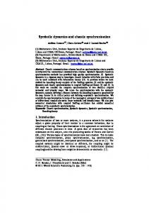
(d) Figure 1. (a) In the absence of top-predator w, a none xycompetitive z dies out in a y-weak, z-weak xyz-web. Initial values: x0 = 0.35, y0 = 0.3, z0 = 0.18, w0 = 0. The parameter values are ζ = 0.01, ²1 = 0.01, ²2 = 0.01, β1 = 0.35, β2 = 0.51, β3 = 0.3, δ1 = 0.6, δ2 = 0.57, δ3 = 0.3. (b) With z = 0, w0 = 0.05, the system settles down to an xyw-cycle. (c) With the addition of z to the same xyw-system, all 4 species tend to a coexisting equilibrium. (d) But with ²1 = 0.065. The system settles down to an xyzwcycle.


X Fold Y Fold Line Z Nullcline W Nullcline Orbit

0.06

0.05

w

0.04

0.03

0.02

0.01

0 0 0.2 0.4 z 0.6 0.35

0.4

0.3

0.25

0.15

0.2

0.1

0.05

0

y

(a) Prey X Predator Y Predator Z Top−predator W

1

Populations

0.8 0.6 0.4 0.2 0

0

0.5

1

1.5

2

2.5 Time

3

3.5

4

4.5

5 4

x 10

(b) 1 0.8

Populations

10

0.6 0.4 0.2 0

0

1000

2000

3000

4000

5000 Time

6000

7000

8000

9000

10000

(c) Figure 2. With parameter values ζ = 0.1, ²1 = 0.1, ²2 = 0.085, β1 = 0.3, β2 = 0.57, β3 = 0.2, δ1 = 0.6, δ2 = 0.52, δ3 = 0.54, the dynamics is a chaotic attractor, projected to the yzw space in (a). The surface is part of the y-nullcline, the red curve on the surface is part of the z-nullcline, and the light green curve on the surface is part of the w-nullcline. The yzw-space shown is also a part of the x-nullcline. These objects are to be explained in subsequent sections. (b) Its time series. With the absence of competitor z (z = 0), the xyw asymptotic state is an equilibrium point as shown in (c) because w is also weak. The creation of this chaos is through the enhancement of the zy-prolificacy: from steady state for small ²1 , to limit cycles via a Hopf bifurcation, the same phenomenon as in Fig.figallweaktimeseries(d), by increasing ²1 modestly, and to chaos by further increasing ²1 .


11

1

Prey X Predator Y Predator Z Top−predator W

Populations

0.8 0.6 0.4 0.2 0

0

500

1000

1500

2000

2500 Time

3000

3500

4000

4500

5000

3000

3500

4000

4500

5000

(a) 1

Populations

0.8 0.6 0.4 0.2 0

0

500

1000

1500

2000

2500 Time

(b) Figure 3. With y and z weak, but w efficient, the system may settle down on either a stable limit cycle or a stable equilibrium point, depending on the initial amount of z. (a) It is attracted to a cycle with an initial value z = 0.02 and parameter values ζ = 0.01, ²1 = 0.005, ²2 = 0.01, β1 = 0.35, β2 = 0.51, β3 = 0.3, δ1 = 0.6, δ2 = 0.62, δ3 = 0.25. (b) It is attracted to an equilibrium with a larger initial value z = 0.15.

3. Numerical Results We now include a short section that will serve as a numerical simulation overview for some of the main results. All simulations are done on Matlab, using the numerical solver ode15s with double precision and BDF (backward differentiation formula) option. Figure 1 demonstrates the phenomenon that top-predation over an dominating competitor can help an extinction-bound competitor compete. Without w, z dies out. With the addition of w > 0, it can coexist with others. It does so at coexisting equilibria for small zy-prolificacy ²1 and at limit cycles as the zy-prolificacy improves via Hopf bifurcation, that the stable coexistence equilibrium becomes unstable, giving way to a cycle in a small neighborhood of the unstable equilibrium. Explaining it holistically, the addition of w increases y’s death rate in a nonlinear fashing, hence decreases its competitive edge against z, and eliminates its total domination over z. Also, increasing z’s competitiveness by increasing its in prolificity against y takes effect only in the presence of w, and destabilizes the dynamics from equilibrium to cycle. Improving the zy-prolificacy further the system can be kicked into chaotic regime even if all predators are respectively weak as shown in Fig.2. It demonstrates that prolificity enhancement alone can have dramatic destabilizing effect. Again, without the top-predation, this scenario cannot take place. Due to its own peculiarity this

12


X Fold Y Fold Line Z Nullcline W Nullcline Orbit

0.06 0.05

w

0.04 0.03 0.02 0.01 0 0 0.2

0 0.1 z

0.4

0.2 0.3 0.6

y

0.4

(a) 1

Prey X Predator Y Predator Z Top−predator W

Populations

0.8 0.6 0.4 0.2 0

0

0.5

1

1.5

2

Time

2.5 5

x 10

(b) 1

Populations

0.8 0.6 0.4 0.2 0

0

0.5

1

1.5 Time

2

2.5 4

x 10

(c) Figure 4. With parameter values ζ = 0.1, ²1 = 0.1, ²2 = 0.004, β1 = 0.3, β2 = 0.57, β3 = 0.2, δ1 = 0.6, δ2 = 0.54, δ3 = 0.3, the dynamics is a rather wild chaotic attractor, showing both in (a) the yzw-projected view and in (b) the time series. Without the z-species (z = 0), the dynamics is an xyw limit cycle as shown in (c) because w is efficient.

is the only case we will not attempt to give a complete analytical explanation to the numerical result. Making w an efficient predator, but keeping y and z weak, there are two possible coexisting attractors. With a small initial amount of z, the solution curve may go


13

to a cycle. This solution curve is near the xyw-cycle, and the z species stays close to the initial condition. However, if a sizable initial amount of z is introduced to the system, it may send the entire system to a coexistence equilibrium. This phenomenon is shown in Fig.3. On one hand, increasing z would seem to enhance w’s predatoriness against y and thus further destabilize the system into a greater cycle. This seemingly counter-intuitive phenomenon can be explained by the Enrichment Paradox. In fact, the competition from z depletes the existing amount of y, decreasing the food supply for the top-predator, hence the opposite to destabilization occurs: the system settles down on a steady state equilibrium instead. In contrasting to the phenomenon of prolificity enhancement to chaos from Fig.2, we can further destabilize such a mild chaos by making w more efficient. The result is presented in Fig.4. There is a greater variability on the attractor than its mild counterpart. In particular, the orbit has different types of sharp zigzag turns, a signature of boom/bust dynamics. Such outbursts of outbreaks and crashes are more evident from the time series plots. We should point out that outbreak/crash dynamics are not limited to chaotic oscillations. They can happen to periodic cycles as well if the reproductive rates are divergently apart. We end this section by noting that all these numerical results will be proved analytically in subsequent sections. 4. Predator-Prey System–Introduction to Singular Orbit Analysis There are 2 issues that are important to ecological consideration: long-term dynamics and short-term trend. Various methods can be used to analyze these problems, not all equal in effectiveness. To motivate the geometric method of this paper, we first give a brief illustration and comparison of these methods. We will do so in the context of the simplest case of one predator and one prey system ¶ µ ¶ µ dx y dy x (7) ζ =x 1−x− , =y − δ1 , dt β1 + x dt β1 + x

which is the xy-subsystem of (3) in the absence of the competitor z (z = 0) and the top-predator w (w = 0). 4.1. Local Linearization. With regard to the simplest long-term dynamics, the system may have a unique xy-equilibrium point, expressed explicitly as x = x e = (β1 δ1 )/(1 − δ1 ) > 0, y = (1 − xe )(β1 + xe ). To determine its local stability, one linearizes the system at the equilibrium point, finds the eigenvalues, and then is lead to the following conclusion (1) The equilibrium state is local stable if and only if the predator y is weak, β1 δ1 /(1 − δ1 ) > (1 − β1 )/2. (2) If y is efficient, 0 < β1 δ1 /(1 − δ1 ) < (1 − β1 )/2, then a small limit cycle is created surround the unstable equilibrium point via Hopf bifurcation. There are a few obvious drawbacks. First, it is only local. Second, it is only about equilibrium point. Third, little can be said about short-term trend in terms of temporal outbreaks and crashes. Last, it is difficult to practically impossible to explicitly solve higher dimensional systems for equilibrium points, or for their eigenvalues, or to apply the Routh-Hurwitz stability criterion (e.g. [21]). To circumvent some of these algebraic difficulties and at the same time to extract just the right amount of information, there is another elementary but effective technique that is, surprisingly, not used more frequently in the literature. We give

14


an illustration of this method in Appendix B since it will be used in various places later. 4.2. Kolmogoroff Method. The second method is based on the following Kolmogoroff’s Theorem of (1936) (c.f. [18]): Theorem: If a system of equations: dx = xf (x, y), dt

dy = yg(x, y), dt

for x ≥ 0, y ≥ 0,

satisfies ∂f ∂f ∂f < 0, x +y < 0; ∂y ∂x ∂y ∂g ∂g ∂g (2) ≤ 0, x +y < 0; ∂y ∂x ∂y (3) There exist constants A > 0, B > C > 0 such that f (0, A) = f (B, 0) = g(C, 0) = 0;

(1) f (0, 0) > 0,

then there exists either a global stable equilibrium point or a global stable limit cycle. It is straightforward to verify these conditions for Eq.(7) with A = xxtr = β1 , B = 1, C = xynl = β1 δ1 /(1−δ1 ). By combining it with the local stability result above we conclude that the existence of a globally stable limit cycle occurs if and only if the predator y is efficient. Although this result gives a complete qualitative description on the long-term dynamics of the system, not much can be said about short-term trend. In addition, the method, as well as the closely related Poincar´e-Bendixson Theorem, is obviously 2-dimensional. We are yet to see any extension of these methods to higher dimensional webs and chains. 4.3. Phase Plane Analysis. The third method is the phase plane analysis, more precisely, the method of vector field analysis using nullclines. The x-nullcline, ζdx/dt = xf (x, y, 0) = 0, of (7) consists of the trivial branch, x = 0, and the nontrivial branch, a parabola y = (1−x)(β1 +x) solved from f (x, y, 0) = 1−x− β1y+x = 0. The importance of considering nullclines is immediately apparent—it tells where a population’s decline turns into a recovery, and vise visa. More specifically, if dx/dt > 0 at a given set of populations x, y, then the prey population x(t) continues to increase at the time. Otherwise it decreases if dx/dt < 0. Therefore, the set of conditions at which dx/dt = 0 usually marks the transition between increase and decrease in population. Exactly the same remarks apply to the y-nullcline, dy/dt = 0, which consists of the trivial branch y = 0 and the nontrivial branch β1 δ1 x β1 +x − δ1 = 0 or x = xynl := 1−δ1 . Also apparent is that the intersections of both variables nullclines give rise to equilibrium points at which neither x nor y changes. Features important for future analysis are: both x-branches intersect at a point (xxtr , yxtr ) = (0, β1 ), referred to as a transcritical point; the maximum point of the 2 1 (1+β1 ) ), which is a fold point. (More information is parabola is (xxfd , yxfd ) = ( 1−β 2 , 4 forthcoming on both transcritical and fold points.) Also dx/dt > 0 for points below the parabola and dx/dt < 0 for points above the parabola, which when translated in practical terms means that with fewer predators the prey is allowed to recover and with an excessive amount the prey must be in decline. The y-transcritical point is y = 0, x = xynl . Also, dy/dt > 0 for points right of the nontrivial y-nullcline, and dy/dt < 0 for points left of it, which implies that an abundant supply in the


15

prey promotes predator’s growth and a depleted stock contributes to its decline. A phase portrait based on these qualitative information is given in Fig.5(a). Because of an apparent vagueness of this equation’s vector field, the method does not always tell the stability of all the equilibrium points, nor the existence of limit cycles. In addition, although the nullcines separate population declines from recovery, they do not foretell the magnitudes by which these events take place, which often are of great practical importance. 4.4. Holistic Approach. The conclusion of the mathematical analysis above can be derived holistically. Starting with the nontrivial x-nullcline, we know that x = 1 is the dimensionless carrying capacity when the system is free of the predator y = 0. As a fixed amount of the predator y > 0 is introduced to system, the prey carrying capacity decreases. The predator-adjusted carrying capacity may disappear at a nonzero level, x xfd > 0, when the predator reaches a critical mass, yxfd , and when the predator concentration is higher than the critical mass, the prey crashes down to zero. This crash crisis may never happen. It depends on whether or not the predator is predatorily strong or weak. More specifically, it depends on whether or not a prey survival threshold is present in the system. For a given level of predation y, xxtd > 0 is called a survival threshold if the prey dies out when its initial concentration is lower than the threshold and grows to its predator-adjusted capacity when its initial concentration is greater than the threshold. Thus the threshold itself is a nontrivial equilibrium state of the prey, if exists, but it is unstable. If it appears above a predator level, yxtr , obviously it must rise higher with a greater concentration of y. Since the threshold increases in y while the y-adjusted capacity decreases in y, they must coalesce at some point, and that point is the crash fold concentrations (xxfd , yxfd ), appearing as a fold point on x-nullcline curve. The crash fold does not appear if a survival threshold never develops. The condition for the existence of the threshold is straightforward: its initial appearance is the intersection of the trivial x-nullcline x = 0 and the nontrivial x-nullcline f (x, y, 0) = 0 such that as y increases the nearby nontrivial x-nullcline increases as well. Specifically, let y = φ(x) = (1 − x)(β1 + x) represent the nontrivial x-nullcline f (x, y, 0) = 0. Then the system develops a x threshold at φ(0) = β1 if dx/dy > 0 which is equivalently 0 < 1/(dx/dy) = dy/dx = dφ(0)/dx. Evaluating dφ(0)/dx = 1 − β1 > 0 implies β1 < 1, which defines the predatory efficiency of y. The predator level y = yxtr at which the threshold reduces to 0 is special. It is referred to as the transcritical point above. The same type of holistic reasoning can be used to describe the y dynamics. But there is one exception on the y-nullcline due to our nonlogistic death rate assumption on y. By the holistic argument, a greater amount of the prey should support a greater amount of the predator, therefore the nontrivial y-nullcline should be an increasing function. It is a vertical line instead for Eq.(7) because of the nonlogistic assumption. Other aspects of the y-dynamics by the holistic argument however are consistent with the analytical argument. In particular, there should be a minimum positive prey mass that only above which can the predator be sustained. Below it, the predator dies out. Above it, the predator population grows. This explains the value xynl and the sign of dy/dt. When combining the descriptions for both prey and predator, we can also derive some qualitative information above the interaction. For example, if the predator

16


needs a greater minimum prey mass to survival than to crash it, i.e., xynl > xxfd , then a crash in x will never materialize if the population concentrations for both x and y are exactly at the levels of crashing x = xxfd , y = yxfd . This is because the crashing concentration in the prey is not enough to sustain an increase in y, and y should be lower than the level of crashing at the next moment of interaction, thus pulling the system away from the crisis of crashing. Such a predator is considered weak (xynl = β1 δ1 /(1 − δ1 ) > xxfd = (1 − β1 )/2) even though it may be predatorily strong β1 < 1. For it to be weak, a number of less desirable factors should be present. The relative mortality rate δ1 = d1 /(b1 p1 ) may be too high, which can result from high death rate d1 , or low birth-to-consumption ratio b1 , or low maximum catch rate p1 , or the relative semi-saturation density β1 = H1 /K is too high. Like the phase plane method, this approach is qualitative in nature, suffering a similar impreciseness of the former. Unlike the phase plane method, it relies on ecological intuition and very little on technicality yet arrives at a comparable level of qualitative understanding. In addition, any technical result should have its holistic interpretation. If such a result proves to be general enough, then its holistic interpretation can become a part of an expanded repertoire of intuitions and principled arguments. The intuitiveness and expansibility of this method are its great strength and appeal. We will use it whenever we can together with the analytical method we introduce next. 4.5. Singular Orbit Analysis. Making up the qualitative shortfall of the last two methods is where the singular perturbation method comes to play under the prolificacy diversification condition: 0 < ζ ¿ 1. It deals with all conceivable types of dynamics problems: from the stability of equilibrium points, to the existence of limit cycles, to the temporal phenomenon of population booms and busts, and to chaos. It does so with a surgical precision in most cases. The results often foretell the dynamics when continued to a moderate parameter range beyond the singular range 0 < ζ ¿ 1 which the method is specifically about. Due to its quantitative nature, the method is inevitably technical, yet always receptive to intuitive and holistic interpretation. When this dual approaches are followed the effort required for comprehension becomes less laborious and the understanding it reaches tends to be optimal. Fast and Slow Subsystems. First the order of magnitude in the course of evolution is explicitly expressed in the dimensionless form (7). For small 0 < ζ ¿ 1, population x changes at a fast order of O(1/ζ) if it is not near its equilibrium (xf (x, y, 0) = 0) already, comparing to an ordinary order of a constant magnitude O(1) for variable y. All non-equilibrium solutions are quickly attracted to a small neighborhood of the stable branches of the x-nullcline: x = 0, y > y xtr or f (x, y, 0) = 0, x > xxfd , the y-adjusted x carrying capacity. Once they are there, the large magnitude O(1/ζ) is neutralized by x’s being near the nullcline state xf (x, y, 0) ≈ 0. Then the y dynamics, which is negligible when x is away from its nullcline state, cannot be neglected further. The subsequent development now evolves according to the ordinary time scale of variable y. There are clearly two phases: the fast development in x followed by the slow evolution in y. In ecological terms, if (x, y) lies above the parabola f (x, y, 0) = 0, then x undergoes a sudden decline or population bust or crash during the x-fast phase. Otherwise, if (x, y) lies below the parabola, then an outbreak or boom in x’s population takes place

17

y


0.6

0.6

0.5

ζ=0

0.5

yxfd 0.4

0.4

y

0.3

0.3

xtr

0.2

yxtr

0.2

0.1

0.2

xpd

ynl

xfd

0

y

0.1

x

x 0

ζ >0

y

0.4

0.6

0.8

1

x

0

0

0.2

0.4

0.6

(a)

0.8

ζ >0

0.6

ζ=0

x−fold point y−nullcline x−nullcline ζ=0.01 ζ=0.04 ζ=0.1 ζ=0.4

β1=0.3 δ1=0.5

0.5

0.5

C

1

(b)

B

0.4

0.4

0.3

0.3

D

A 0.2

0.2

0.1

0.1

0

0

0.2

0.4

0.6

(c)

0.8

1

0

0

0.1

0.2

0.3

0.4

0.5

0.6

0.7

0.8

0.9

1

(d)

Figure 5. (a) A typical vector field of the xy-system. The xcomponent of the vector field points towards the solid branches of the x-nullcline and away from the dashed ones. Similar convention is used for branches of the y-nullcline. Species y is weak iff xxfd < xynl . (b) A typical case of weak y and the stability of the equilibrium point by singular orbit analysis. The green curve is a relaxed orbit for 0 < ζ ¿ 1. See text for the derivation of yxpd on the phenomenon of Pontryagin’s delay of loss of stability at which a boom in x population occurs although the recovery starts after its crossing the dashed threshold on the parabolic x-nullcline near yxtr . (c) A typical case of efficient y, the existence of a singular limit cycle and its relaxed cycle for 0 < ζ ¿ 1. (d) The effect of relative prolificacy is shown.

instead. In contrast, during the y-slow phase the y population undergoes a slow decline if there is not enough prey supply or a slow rebound otherwise. These fast and slow dynamics can be captured both qualitatively and quantitatively at the limit ζ = 0 to equation (7). More precisely, setting ζ = 0 in Eq.(7) results in ¶ µ ¶ µ dy x y , =y − δ1 . (8) 0=x 1−x− β1 + x dt β1 + x

18


It is a system of algebraic and differential equations. It can also be viewed as a differential equation on the x-nullcline manifolds: x = 0 and f (x, y, 0) = 0. It captures the dynamics of the slow phase in the sense that if (xζ , yζ )(t) is a segment of a solution of Eq.(7) for ζ > 0 that is near the x-nullcline during the y-slow phase, then the limit (x0 , y0 )(t) = limζ→0 (xζ , yζ )(t) must satisfy the limiting equation (8). For this reason, we call (8) the slow subsystem of Eq.(7) and view Eq.(7) in the slow time scale of variable y, which in fact was originally scaled against the maximum reproductive rate of species Y . In practical terms, the prey always adapts to its predator-adjusted carrying capacity one step ahead of any change in the concentration of the predator because it always out-reproduces its predator. Similarly, if we change the time variable of Eq.(7) from t to τ = t/ζ, then the equation becomes µ µ ¶ ¶ x dx y dy (9) =x 1−x− = ζy − δ1 . , dτ β1 + x dτ β1 + x The time scale is set according to that of variable x. Setting ζ = 0 in the equation above gives rise to ¶ µ dy y dx , =x 1−x− = 0. (10) dτ β1 + x dτ It is a 1-dimensional system in the fast variable x with y frozen as a parameter. Again, the equation captures the dynamics during the x-fast phase in the same sense as equation (8) does to the y-slow phase: the limit (x0 , y0 )(τ ) = limζ→0 (xζ , yζ )(τ ) must satisfy equation (10) if (xζ , yζ )(τ ) is a solution segment of Eq.(9) during the x-fast phase. For the obvious reason, we call Eq.(10) the fast subsystem of Eq.(7) and view Eq.(9) in the fast reproductive scale of the prey x. In practical terms, if the prey is not in its stable state, whether that is the predator-adjusted carrying capacity or the wipe-out state x = 0, it will quickly converge to it if the reproductive rates are divergent in the prey’s favor. In terms of terminology, solutions as well as orbits of Eq.(8) are described by adjective slow whereas those of Eq.(10) by fast. These orbits are also referred to as singular orbits as well as their natural concatenations. By natural concatenation it means the following. A fast orbit of Eq.(10) must asymptotically approach a point on the x-nullcline x = 0 or f (x, y, 0) = 0. From that point, a slow orbit of Eq.(8) develops on the x-nullcline. The union of these two orbits oriented in the common sense of time is one case of the natural concatenation of fast and slow singular orbits. In practical terms, for example, it may capture the transitional events from a population boom in x to its slow decline and y’s slow rise, or a bust in x to its slow recovery and y’s slow decline as seen in Fig.5(b,c) for concatenated singular orbits and their perturbed orbits. The criterion for determining stable branches of the x-nullcline is ∂(xf )/∂x < 0 at the nullcline point, which in turn translates into (11)

f |{x=0} < 0 at the trivial branch x = 0 fx |{f =0} < 0 at the nontrivial branch.

Reversing the sign for unstable branches. Setting them to zero for transcritical points and fold points respectively. These criteria are listed here for future reference. Mechanism of Outbreak. The remaining case of natural concatenation is associated with mechanisms by which singular orbits jump away, rather than into,


19

nullclines. In practical terms, it deals with sudden temporal transitions of population: a slow decline and a slow recovery respectively in population y and x followed by a sudden outbreak in x, or a slow build up and a slow decline respectively in y and in x followed by a sudden crash in x. Because of their theoretical importance to the singular orbit analysis both qualitatively and quantitatively, and because of their practical importance to sharp temporal shifts in population, we give a detailed illustration to each scenario below. The first case takes place near the transcritical point (0, yxtr ) = (0, β1 ) at which two branches of the x-nullcline, x = 0 and f (x, y, 0) = 0, intersect. The exposition below gives an illustration to the relation between the onset of prey outbreak and the initial predator concentration preceding the outbreak. Let x = a, 0 < a < xynl , xxfd be any line sufficiently near the y-axis. Let (a, y1 ) be any initial point that is on the line and above the parabola. Let (xζ (t), yζ (t)) be the corresponding solution of the perturbed system (7) with 0 < ζ ¿ 1 and with the initial point. The solution must move down because x = a y˙ < 0 for it is to the left of the nontrivial y-nullcline. It moves leftwards above the unstable parabola xnullcline until it crosses the parabola at a point (xp , yp ), 0 < xp < a, β1 = yxtr < yp at which the solution curve is vertical. It then moves down but rightwards since now the x is in the recovery mode x˙ > 0. A finite time Tζ > 0 later it intersects the cross section line x = a at a point denoted by (a, y2 (ζ)). In general the second intercept y2 (ζ) depends on ζ. Now integrating along the solution curve we have Z Tζ Z y2 (ζ) ζ x˙ ζ ζ x˙ ζ a dt = dyζ 0 = ζ ln x|a = x x ζ ζ y˙ ζ 0 y1 Z y2 (ζ) f (xζ , yζ ) = dyζ . y ζ g(xζ , yζ ) y1 Taking limit ζ → 0 on both sides of the equation above, using the facts that x ζ → 0, xp → 0, yp → yxtr = β1 and the notations that y1 = y, y2 (ζ) → yxpd , yζ → s, we obtain the integral equation Z y f (0, s, 0) ds = 0 sg(0, s, 0) yxpd for variables y and yxpd . In practical terms, y approximates the value followed by a collapse in x starting at the initial (a, y) and yxpd approximates the value that immediately precedes a outbreak in x. Because the integrant f (0, s, 0)/sg(0, s, 0) has opposite signs for s > yxtr and for s < yxtr , we immediately conclude the following qualitative property: the greater concentration y at the state of the xcollapse the lower concentration yxpd it reaches before the x-outbreak can take place. We also have its quantification: yxpd is the value so that the two areas bounded by R y f (0,s,0) R yxtr f (0,s,0) the integrant graph are equal: yxtr sg(0,s,0) − sg(0,s,0) ds. Notice that the ds = yxpd branch x = 0, y < yxtr is effectively unstable for the fast x-subsystem Eq.(10). The above phenomenon that singular orbits develop beyond a transcritical point, continue along the unstable part of a nullcline before jumping away is called Pontryagin’s delay of loss of stability. The case illustrated is for the type of transcritical points at which the fast variable goes through a phase of crash-recovery-outbreak. In other cases of generalization, they may be responsible for a reversal phase for the fast variable. However, all the known PDLS cases of our XY ZW -model are

20


of the crash-recovery-outbreak type described above. We often call them outbreak PDLS points. Predatory Efficiency and Mechanism of Bust. The remaining case is associated with a slow build-up and a slow decline in y and x respectively followed by a sudden crash in x. It happens only when the predator y is efficient 0 < xynl < xxfd . We adopt a similar set-up and steps as for the transcritical turning point above to describe the crash mechanism. First let x = a with xynl < a < xxfd instead and let (a, y1 ) be any initial point from x = a so that y1 < yxfd = (1 − xxfd )(β1 + xxfd ) instead. Because it is below the parabola, the perturbed solution (xζ , yζ )(t) moves right-up, crosses the stable parabola x-nullcline vertically, moves left-up and hits the cross-section line x = a again at a point denoted by (a, y2 (ζ)). Use the exact orbit-integral-to-ζ-limit argument above to get a similar integral equation Z

y2 (0) y1

f (x0 , y0 , 0) dy0 = 0, y0 g(x0 , y0 , 0)

with limζ→0 (xζ , yζ ) = (x0 , y0 ) being the y-slow singular orbit on the parabola f (x0 , y0 , 0) = 0. Since y2 (ζ) > yxfd for ζ > 0, we must have y2 (0) ≥ yxfd . The equation above does not hold if y2 (0) > yxfd because the integrant would be strictly negative for integration interval yxfd < y0 < y2 (0). Hence we conclude that y2 (0) = yxfd , independent of the any initial concentration (a, y1 ) with y1 < yxfd . In practical terms, the collapse in x’s population will occurs invariably whenever y’s population reaches the crashing fold concentration yxfd . Competitiveness. By definition (see Appendix A), predator y is competitive iff the x-attractor at the carrying capacity (1, 0) is unstable with respect to the xysystem, which in turn requires y to grow per-capita ((1/y)dy/dt = g(x, y, 0) > 0) near that point, i.e., g(1, 0, 0) = (1/(β1 + 1) − δ1 > 0. Solving this inequality gives rise to δ1 < 1 and β1 δ1 /(1 − δ1 ) < 1, which is equivalent to 0 < xynl = β1 δ1 /(1 − δ1 ) < 1, that is the minimum concentration of x needed for y to grow should be no greater than the prey carrying capacity. If y is noncompetitive, then either xynl = β1 δ1 /(1 − δ1 ) < 0 in which case δ1 > 1 implying that y dies out faster than it reproduces, or xynl = β1 δ1 /(1 − δ1 ) > 1 implying y is weaker still in terms of predation efficiency. In either case, (1, 0) is globally stable and y dies out eventually. The information that y is competitive is enough to conclude its survivability. This can be taken as a rudimentary rule for competitive survivability. Although the argument is rather simplistic for this 2-dimensional case, it will become increasingly more substantial as more species are taken into consideration. Classification. With most necessary ingredients in place for the method of singular orbit analysis we now complete our showcase for the predator-prey model Eq.(7). If y is noncompetitive, it dies out eventually. If it is competitive, there are 2 subcategories to consider: weak and efficient predations. For the weak case, xxfd < xynl < 1, all non-equilibrium singular orbits converge to the coexisting steady state as shown in Fig.5(b). For the efficient case, xxfd > xynl > 0, all nonequilibrium singular orbits converge to the limiting singular cycle ABCD as shown in Fig.5(c). We note that when y is weak, all singular orbits eventually settle down on and never leave the stable branch of the nontrivial x-nullcline f (x, y, 0) = 0, x xfd < x < 1. That is, this branch is flow invariant. The practical interpretation is that weak


21

predation leads to long term steady supply in the prey. This intuitive argument will also be used to derive some useful conclusions later. Enrichment Paradox. The conclusion that efficiency leads to population cycle is the generalized principle of the well-known Enrichment Paradox by Rosenzweig ([25]). In fact, increasing the prey carrying capacity K decreases the dimensionless semi-saturation parameter β1 = H1 /K, which in turn can drive the predator into efficiency regime: xynl = β1 δ1 /(1 − δ1 ) < xyfd = (1 − β1 )/2. Prolificacy Duality. Prey-to-predator prolificacy has no long term effect for weak y as all solutions converges to the coexisting equilibrium point. Short term outbreak and collapse can occur depending on the current state of the species in their phase space, see Fig.5(b). More specifically, if the prey x is in a decline phase x˙ < 0, increasing its prolificity has a counter-intuitive effect. Instead of increasing its number, it crashes to the bottom even faster. The predator stands alone to rip all the benefit: Y = rK p1 y and the prey has nothing to gain against its fixed carrying capacity: X = Kx. The only circumstance in which increasing its prolificity is self-beneficial is when the prey is in a recovery mode (x˙ > 0). In such a case, it quickly reaches its predator-adjusted carrying capacity—the stable branch of the parabolic x-nullcline f (x, y, 0) = 0. Prey’s over prolificity is a double-edged sword. Important principles that can be derived from here is that periodic outbreaks and collapses are unavoidable under the combination of predatory efficiency and preyto-predator over-prolificity. Even more surprising is the scenario of the phenomenon of prolificity-to-chaos as we have seen in the numerical simulation of Fig.2 and in theory later. Persistence. The importance of this analysis at the limit ζ = 0 lies in the fact that all the singular asymptotic structures will persist for small (often moderate ζ in practice) 0 < ζ ¿ 1! The theory of persistence has been well-developed, c.f. [23, 22, 10, 9, 1, 27, 19, 4], which enables us to focus our attention primarily on singular orbit structures in applications if the main purpose is to understand the underlining dynamics. For this reason, we will only make sparse comments on persistence questions throughout the paper. Prolificacy Reversal. A case can be made that the method of singular orbit analysis is far superior than other methods described. The only drawback seems to be the lack of a treatment for large ζ À 1. A closer examination shows however the drawback is not as significant as it first seems. First, the practical interpretation of large ζ > 1 implies that the predator out-reproduces its prey. Such rate-reversal systems are less common than their rate non-reversal counterparts. Second, if the predator has the potential to multiply faster than its prey, then Verhulst’s logistic growth assumption must be incorporated into predator’s model by assuming that Y ’s per-capita death rate is density dependent: d + d 0 Y . Upon non-dimensionalizing, the y takes this form dy/dt = y(x/(β1 + x) − δ1 − δ0 y). For large ζ À 1, the resulting model is again a singular perturbed system for which y is fast and x is slow. The nontrivial y-nullcline is monotone increasing function of x with y saturation: y = (x/(β1 + x) − δ1 )/δ0 , consistent with our earlier holistic prediction on the qualitative behavior of the prey induced predator equilibrium. The same singular orbit analysis can be applied again. Without Verhulst’s assumption, application of the singular orbit analysis will fail. More specifically, since the nontrivial y-nullcline x = xynl would be a vertical line parallel to all y-fast singular orbits, at the limit ζ = ∞, all fast y-orbits for x > xynl would fly to infinity without

22


bound, which would leads to an ecological absurdity that a fixed amount of prey sustains any ever increasing amount of predator. The failure does not come from the method rather than the unrealistic assumption of a nonlogistic growth on the fast reproducing predator y. We will not treat the rate-reversal models any further in this paper. We conclude this subsection by pointing out that a summary of the singular orbit analysis methodology, in particular, the analysis of sharp temporal falls and rises involving multiple folds and transcritical threshold points, is given in Appendix C for future reference for higher dimensional systems which we will consider below. 5. Competition Exclusion: XY Z-Web In this section, we will set up the x-dynamical range for which the main analysis of Sec.7 is to be carried out. In doing so we will highlight some known results of the xyz-web and inevitably some open problems as well. As demonstrated by the simple predator-prey xy-system in the previous section, this method follows these steps: (1) separate the nullclines into typical configurations according to web characteristics in terms of competitiveness, efficiency, and prolificacy which usually can be quantified mathematically; (2) classify typical short term and long term singular orbit structures for each category; (3) demonstrate persistence of singular structures for the perturbed system, which is optional for this paper. In carrying out task (2), we will break the system down to fast and slow subsystems, and piece together the higher dimensional singular orbits from the lower dimensional and always simpler ones through concatenation via crash fold and outbreak PDLS points. For the xyz-system dy dz dx = xf (x, y, z), = yg(x, y, 0), = ²1 zh(x, z), ζ dt dt dt all the nullclines are now surfaces, each always consists of two branches: the trivial and the nontrivial ones. In singular perturbation terminology, we also refer to these surfaces as slow manifolds whenever appropriate. While the ζ-fast subsystem is still 1-dimensional, the ζ-slow subsystem on the other hand is 2-dimensional, which in turn is singularly perturbed if ²1 → 0 is allowed. We will use similar ideas and techniques from Sec.4. The only difference is to apply them in multi-dimensions. The nontrivial x-nullcline, f (x, y, z) = 0, consists of equilibrium states for the xequation when y, z are kept constants. The stable equilibrium state is the predators yz-adjusted carrying capacity. It must decrease with increase in either y or z or both. A crash fold point developed at a given pair of (y, z) if at (y, z) there is an adjusted capacity x which disappears upon any small increase either in y or z. Again the existence of crash fold points for a given concentration in y, z depends on whether or not survival thresholds develop for the prey. The condition for the existence of threshold requires that at the intersection of the nontrivial branch and the trivial branch of the x-nullcline, the prey concentration increases with increase in y, z along the nontrivial branch. Mathematically, it equivalent to ∂x/∂y > 0, ∂x/∂z > 0 with x, y, z satisfying f (x, y, z) = 0, and partial derivatives evaluated at points satisfying f (0, y, z) = 0. The crash fold curve should have the following properties. First, if y is increased, then a decreased amount of z is only needed to crash x. Therefore, on the yz-plane, the curve is a decreasing function of z when y is increased and vis


23

x−nullcline 1

x−nullcline

1

0.9

0.9

co−existing cycle

0.8

0.8

S

0.7

0.7 0.6

x

0.6

x−fold curve

x

0.5

0.5

0.4

0.4

z−nullcline

0.3 0.3

0.2 0.2

0.1

y−nullcline

0.1

0 0 0.1

0.3 0.2

z

0.4 0 0

0.2 0.3

y

0.4

x−transcritical line

0.1

0.2

0.1

y

0

0.3

0.4

(a)

z

0.3

0.2

0.1

0

0.4

(b) 0.45

ε =0

x−fold curve

1

0.4

1

ε >0 1

0.9

0.35

x−transcritical line

0.8

0.3 0.7

0.25

y−nullcline

x

z

0.6 0.5

0.2 0.4

0.15

0.3 0.2

0.1

z−nullcline

0.1

0.05 0 0

0.1

0.2

0.3

y

0.4

0

(c)

0.05 0.1

0.15 0.2

0.25 0.3

z

0.35 0.4

0

0

0.05

0.1

0.15

0.2

y

0.25

0.3

0.35

0.4

0.45

(d)

Figure 6. (a) The x-nullcline, with the stable branches outlined in solid red and unstable branches by dash red. Phase lines of the x-fast flow are in black. (b) When both y, z are efficient and competitive, co-existing cycle must exist. The co-existing cycle is shown for parameter values: ζ = 0.1, ²1 = 1, β1 = 0.25, β2 = 0.325, δ1 = 0.5, δ2 = 0.45, for which it can be verified numerically that y, z are competitive. (c) A 3-d view of the nullcline surfaces is shown for the same parameter values as in (b) except for β2 = 0.25, δ1 = 0.75, δ2 = 0.775, for which both y, z are weak. (d) A reduced 2-d phase portrait view. A case of non-competitive z is shown. Solid blue vector field and curve for a perturbed case ²1 > 0 and dotted black curves for ²1 -singular orbits. Both give the same y-dominant conclusion. versa. Let zxfd |{y=0} denote the amount of z that is needed to crash x when y = 0 and xxfd |{y=0} the corresponding single predator-adjusted x-capacity, and similar notation for yxfd |{z=0} and xxfd |{z=0} . If both single predator-adjusted crashing capacities are the same xxfd |{z=0} = xxfd |{y=0} , then intuitively the joint yz-adjusted crashing capacity should remains the same. If they are different that one is higher than the other, then the crash fold curve xxfd decrease from the higher crash capacity to the lower one. For example, suppose y can crash x at higher concentration of

24


x than z does. Then y puts a greater predatory pressure on x than z does. Since we know it requires a smaller amount of y to crash x if z is increased, then it is reasonable that the new predator-adjusted crashing capacity should be lowered. These properties, although intuitively reasonable, require technical justification which we give below. It is important to make use of the fact that the nontrivial x-slow manifold, y z f (x, y, z) = 1 − x − − = 0, β1 + x β2 + x is linear both in y and z. Thus, by a standard introduction of a parameter, α, this surface can be alternatively expressed as follows (12)

y = α(1 − x)(β1 + x), z = (1 − α)(1 − x)(β2 + x) for 0 ≤ x ≤ 1 and 0 ≤ α ≤ 1,

which offers many practical conveniences below. The transcritical curve is the joint solution to the two x-slow manifolds x = 0, f (x, y, z) = 0. Using the parameterization (12) we have for the transcritical curve as ¶ µ y β2 , with 0 ≤ α ≤ 1, x = 0. (13) y = αβ1 , z = (1 − α)β2 = 1 − β1 It is a line with end points: (x, y, z) = (0, β1 , 0) at α = 1 and (x, y, z) = (0, 0, β2 ) at α = 0 which are the transcritical points for the respective xy-system and the xz-system as special cases. The x-fold curve is where the manifold f (x, y, z) = 0 comes in tangent to the horizontal x-fast flow lines. Hence it necessarily satisfies these two equations f (x, y, z) = 0, fx (x, y, z) = 0 simultaneously as we have already pointed out in (11). Using the parameterization (12) again together with the additional equation y x fx (x, y, z) = −1 + + = 0, 2 (β1 + x) (β2 + x)2 we obtain after eliminating the parameter α the x-fold curve: (2x − 1 + β2 )(β1 + x)2 β2 − β 1 (2x − 1 + β1 )(β2 + x)2 (14) z= β1 − β 2 1 − max{β1 , β2 } 1 − min{β1 , β2 } for 0 iff (y, z) is to the left side y=


25

of the transcritical line f (0, y, z) = 0.) Similarly, the yz-adjusted capacity on the nontrivial x-slow manifold f (x, y, z) = 0 is stable (since fx (x, y, z) < 0) and the threshold part is unstable (since fx (x, y, z) > 0). A typical sketch for the x-nullcline surfaces is given in Fig.6(a). All singular orbits must intersect the x-stable branches. Of the last two, all singular orbits must either visit or stay on the stable nontrivial branch. This is because with depleted food source x ≈ 0, y, z will decrease and eventually across the x rebound/outbreak transcritical line (13) and jump up onto the x-capacity branch, guaranteed by the principle of Pontryagin’s delay of loss of stability. Hence, any singular xyz-attractor must either contain a part of the x-capacity manifold or stay there if x cannot be crashed. We now set up in detail an important part of the framework for this paper: joint weak predation by y and z. Recall that if y is weak, then its required minimum prey density for grow, xynl , is greater than the amount to crash x, i.e. xynl > xxfd |{z=0} . So it alone cannot crash x dynamically on the y-adjusted x-capacity. Similarly, z is weak provided xznl > xxfd |{y=0} . Joint weak predation assumption requires more than individual weakness. We assume instead that everywhere along the crash fold curve, none of the predators can grow. In other words, once the singular orbit reaches the predator-adjusted carrying capacity, crash in the prey population is not possible. We also refer to this assumption as yz-weak predation assumption. In technically terms, the nontrivial y-nullcline and z-nullclines are two parallel planes, x = xynl =

β2 δ2 β1 δ1 , x = xznl = , 1 − δ1 1 − δ2

and the yz-weak predation requires both planes lie above the x-fold curve. Because the x-fold ranges in x only in the interval (1 − max{β1 , β2 })/2 < x < (1 − min{β1 , β2 })/2 by (14), this setup holds iff the y, z nullcline values xynl , xznl are greater than the upper end x-value of the fold: min{xynl , xynl } = min{

βi δi 1 − βi 1 − min{β1 , β2 } } > max{ }= . 1 − δi 2 2

Since weak y, z automatically implies xynl > (1 − β1 )/2 and xznl > (1 − β2 )/2, the condition above reduces to xynl > (1 − β2 )/2 and xznl > (1 − β1 )/2. In this setting the stable nontrivial x-slow manifold is invariant for the ζ-slow yz-flow. Because we will almost exclusively work with this surface of predator-adjusted carrying capacity, we will denote it by S = {f (x, y, z) = 0, fx (x, y, z) < 0}. Also we denote by D its projection to the yz-plane, that is the region bounded the y, z axises and the yz-projection of the x-fold curve. Because of its invariance, the ζ-slow subdynamics on S is only 2-dimensional and we will take the advantage by conducting our analysis on the projected yz-plane, as shown in Fig.6(c,d). We only give a practical argument to justify the vector field plot of Fig.6(d): For y below its nullcline, it is relatively small. Its food supply is relatively abundant and therefore y will grow. For y above its nullcline, it will decline. Similar argument applies to z. We note that the y-nullcline and z-nullcline are two parallel planes, and so they do not intersect in general unless xynl = xznl . We conclude immediately that there does not exist any co-existing equilibrium point except xynl = xznl . The Competition Exclusion Principle is in large part because of this fact.

26


Table 2. Summary on Coexistence Competitor z Eq.(3) with w = 0 WC WNC EC Competitor y WC NA y Dominant Co-Cyc.∗ WNC NA Open EC Co-Cyc. ENC NA — Not Applicable Co-Cyc. — Coexistence in limit cycles WC — Weak and Competitive predator WNC — Weak and Noncompetitive predator EC — Efficient and Competitive predator ENC — Efficient and Noncompetitive predator Open — Never investigated ∗ — Open question on persistence proof

ENC Open Open Open Open

To compensate the almost artificial treatment on competitiveness of Sec.4, we give here a more substantial and genuine treatment on the subject. Because both y and z are weak, the xy-attractor and xz-attractor are equilibrium points. Therefore y is competitive iff, by definition, the xz-equilibrium point is unstable with respect to the xyz-system, iff y can still grow per-capita near the xz-capacity equilibrium, (dy/dt)/y = g(x, y, 0) > 0, and specifically g(xznl , 0, 0) = xznl /(β1 + xznl ) − δ1 > 0. Solving the last inequality we have xznl >

β1 δ1 = xynl . 1 − δ1

We already pointed out early that the smaller the value xynl the more efficient y is. Hence this inequality above can be interpreted as that y is more competitive than z because and only because it is relatively more efficient. This relation automatically concludes y and z cannot be both competitive when they are both weak. Because there are no xyz-equilibrium points and the yz-dynamics on S is 2-dimensional, the xy-equilibrium point is globally attracting, killing off z eventually. Therefore the necessary condition for coexistence requires at least one of the two predators to be efficient. As a sufficient condition, coexistence occurs if both predators are competitive, i.e. both the xy- and the xz-attractors are xyz-unstable. For example if the xz-attractor is a limit cycle in the case of efficient z, then y is competitive provided this cycle is xyz-unstable asymptotically. Equivalently, Z Tc g(xc (t), 0, zc (t))dt > 0, 0

where (xc (t), 0, zc (t)) denotes the xz-limit cycle and Tc the xz-cycle period. In practical terms, at each point of the cycle, the sign of g(xc (t), 0, zc (t)) tells whether y increases or decreases, and g(xc (t), 0, zc (t)) is the magnitude of per-capita rate of change at this point t. Then the averaged per-capita net change over the period T c is precisely Z Tc 1 g(xc (t), 0, zc (t))dt. Tc 0


27

0.5

x−nullcline

0.5

0.45

y−nullcline

0.4

0.4

0.3

y

y

0.35 0.3

0.25 0.2

0.2 0.1

0.15

w−nullcline

0.1

0 0

0.05 0.2

0 0

0.4 0.6 0.1

0.8

x

0.05 1

0

w

0.15

0.5

x

1

0

(a)

0.02

0.04

0.06

0.08

w

0.1

(b)

Figure 7. (a) A sample of computer generated x, y, w nullclines in the xyw-space. (b) An xyw-slow cycle as y is weak and w is efficient. Parameters values: ζ = 0.1, ²1 = 0.1, ²2 = 0.1, β1 = 0.3, β2 = 0.57, β3 = 0.2, δ1 = 0.6, δ2 = 0.54, δ3 = 0.5, and z = 0. Hence, if the integral is positive, then the net per-capita change in y along the cycle is a gain, and y grows as a group. See Appendix A for technical reasoning. Limit cycle is the only known form of coexistence. This result is the complimentary part of our current understanding on the Competition Exclusion Principle. Last, we remark that each predator can be classified into 4 categories in terms of efficiency and competitiveness. Therefore there are 16 categories for 2 predators. Excluding symmetrical duplications and impossible combinations there are 8 distinct cases left, of which 5 cases have never been investigated. The status is summarized in Table 2. We refer to [15] for a geometric treatment of both y, z efficient and competitive case. 6. XY W -Chain with Weak Y We consider in this section the xyw-chain free of the mid-lateral competition β1 δ1 1 . < xynl = 1−δ (z = 0) under the assumption that y is weak: xxfd = 1−β 2 1 Taking a similar approach as in the previous section, we first consider the nullcline surfaces. The nontrivial x-slow manifold is a parabola cylinder parallel to the w-axis: y = (1 − x)(β1 + x), for 0 ≤ x ≤ 1. It is the same x-nullcline as for the xy-system extended in the positive w-axis direction. Because x is in direct interaction only with y, the predator-adjusted x carrying capacity therefore depends only on y as well. All the properties about the x-nullcline can be directly borrowed from Sec.4. Its fold line and transcritical lines are respectively: (x, y) = (xxfd , yxfd ) = ((1 − β1 )/2, (1 + β1 )2 /4), and x = 0, y = ytrn = β1 , for w ≥ 0. Similar, the attracting branches of the x-slow manifold are the parabola between xxfd < x < 1 and the trivial manifold x = 0 above the transcritical line y > β1 . Also, since y is weak, the former is globally attracting and invariant as weak predation does send the prey crashing through the fold boundary of the predator-adjusted carrying capacity. Without introducing new notation we again denote this manifold by S.

28


The nontrivial y-nullcline surface is ¶ µ x − δ1 (β3 + y). w= β1 + x Since y > 0, it imposes the range x/(β1 + x) − δ1 > 0 which in turn implies x > β1 δ1 /(1 − δ1 ) = xynl . The holistic explanation is that a greater minimum prey density is required in order for y to grow when itself is preyed upon from w. As always, to the side of unbounded top-predator w, the prey y decreases in population because the predatory pressure from w is too great. The nontrivial w-nullcline k(y) = 0 is a plane parallel to the xw-plane: y = ywnl =

δ3 β3 1 − δ3

Below the plane (not enough prey y), w˙ < 0, and above the plane w˙ > 0. To determine the ζ-slow dynamics on the invariant 2-dimensional manifold S, we consider the reduced y-nullcline on S, namely the xw-adjusted y equilibrium state. Denote by γ = {g = 0} ∩ {f = 0} the intersection of the nontrivial y-nullcline with S. Because y is weak, the xy asymptotical state is the xy equilibrium point. This w-adjusted xy-equilibrium decreases in y with increase in w, moving away from the x crash fold. The top-predator w can crash the y population at a nonzero concentration if w is efficient so that a nonzero survival threshold for y develops at the intersection of the trivial y-nullcline y = 0 and the nontrivial one g(x, y, w) = on the x-nullcline f (x, y, 0) = 0. Use the same property that the threshold increases in y with increase in w, we will derive in Appendix D (a special case of Proposition 12.1 with z = 0) that under the condition ¶ µ (β1 + 1)3 1 (15) β3 < − δ1 β1 β1 + 1 a nonzero y threshold develops and there exists a unique y crash fold point on w = γ(x) in [xynl , 1]. Notice that the y-crash fold develops only when β3 is relatively small, the predatory efficiency requirement on the part of w, consistent with the analysis of Sec.4. The crash fold point separates γ into two parts: the top part contains the w-adjusted xy capacity equilibria. Its y component decreases with increase in w. It is y-stable. The bottom part, if w is predatory efficient, is yunstable. The intersection with the trivial branch y = 0, x = 1, y = 0, wytr = γ(1), is the only y-rebound/outbreak transcritical point. Denote the fold point’s y-coordinate and w-coordinate by yyfd and wyfd . Last, the w-nullcline surface on the S is again a straight line. Putting all these elements together, we see that the ζ-slow phase portrait on S is qualitatively the same as the predator-prey xy-system of Sec.4. The reduced system is also singularly perturbed by ²2 , the wy prolificacy parameter. See Fig.7(b). Dynamically, w is weak if yyfd < ywnl < yxfd , and the corresponding equilibrium point attracts all ²2 -singular orbits. W is efficient if 0 < ywnl < yyfd and in which case a limit cycle appears, and its singular counterpart attracts all ²2 -singular orbits. Since it does not contain fast x outbreaks and crashes through the x crash fold, we all call this type of cycles the x-slow cycles which when restricted on S are y-fast cycles. Also all the ²2 -prolificacy induced boom and bust dynamics in y are completely parallel to the xy case of Sec.4.


29

In closing we point out that the food chain dynamics can become extremely complex for efficient predator y. There are 4 known types of chaotic attractors with efficiency-efficiency combination for y and w, conforming yet again the principle that efficiency leads to complexity, see [5, 6, 7, 8] for details. We also point out that the xslow cycles and the equilibrium points all persist for small 0 < ζ ¿ 1, 0 < ² 2 ¿ 1, since their hyperbolicity can be verified and therefore the persistence results of [10, 1] can be applied. 7. Main Results: Dynamics of Weak Y, Z XY ZW -Web We now consider the full xyzw-web. For convenience the full system is recalled from Eq.(3)below  µ ¶ z   ζ dx = x 1 − x − y − := xf (x, y, z)    dt β1 + x β2¶+ x  µ   dy w x   =y − − δ1 := yg(x, y, w)  dt β + x β +¶y 1 3 µ (16) x dz   = ²1 z − δ2 := zh(x)    dt β 2  µ +x ¶   y dw   = ²2 w − δ3 := wk(y)  dt β3 + y

We only consider in this paper the seemly simplest case: trophic diversified prolificacy for both xyw and xz chains and joint yz-weak predation. We will mostly use holistic and geometrical arguments and supplement them by technical analysis from Appendix E. Dimension Reduction. The nontrivial x-nullcline f (x, y, z) = 0, its crash-fold, stable, and unstable branches are the same for the full system as for its xyzsubsystem because w does not directly interact with x. We use the same notation S as in the previous sections for the stable branch of the nontrivial x-manifold. It is the same as before except that it is a 3-dimensional solid in the xyzw-space. We know from Sec.5 that without w, the solid S is invariant for the ζ-slow yzflow if y, z are yz-weak. As argued before, because of the yz-weak assumption, y, z are in a decline mode near the x-fold state, hence prevent x from crashing, which in turn implies the surface S ∩ {w = 0} is invariant for the ζ-slow yz-subsystem. With the presence of w predation, y must be in a steeper decline near the x-fold than without, and for the same reason crash in x never take place and the solid S is invariant for the full ζ-slow yzw-system. Any point (x, y, z, w) from the solid S can be expressed by a relation with x as a function x = q(y, z) of y, z. It means for each level of y, z predation, there is a unique yz-adjusted carrying capacity of the prey, which by definition defines the stable nontrivial branch of the x-nullclline. Also, the function q is decreasing in both y and z because the yz-predation pressure depresses the adjusted prey steady state. On the trivial x-slow manifold x = 0, the transcritical points for the full web remain the same as for the xyz-web. All ζ-singular orbits must cross it and jump to the solid S at some x-outbreak PDLS points for the reason that x and w do not directly interact with each other. Therefore, all nontrivial ζ-singular orbits eventually settle down into the invariant solid S. And we only need to consider the 3-dimensional yzw-slow system in S. A dimension reduction is now obtained.

30


Mathematically, S is defined by f (x, y, z) = 0, fx (x, y, z) < 0. Because of the hyperbolicity fx (x, y, z) < 0, variable x can be solved by the Implicity Function Theorem as a function of q(y, z) from f (x, y, z) = 0 with (y, z) from the same set D as in Sec.5 that is bounded by the y, z axis and the x-fold curve projected onto the yz-plane. Also q is a decreasing function in both y and z: qy (y, z) < 0, qz (y, z) < 0 (see Appendix E). The ζ-slow yzw-system in S is then expressed explicitly as follows:  ¶ µ w q(y, z) dy   =y − − δ1 = yg(q(y, z), y, w)    dt β1 + q(y, z) β3 +¶y  µ  dz q(y, z) (17) = ²1 z − δ2 = zh(q(y, z))  dt β  µ 2 + q(y, z) ¶   dw y   = ²2 w − δ3 = wk(y)  dt β3 + y

Z-Dominant Dynamics. If z is xyz-dominant (h(xynl ) > 0), y dies off eventually even without top-predator’s presence. The weaker competitor would meet its extinction-bound fate sooner with w > 0, and take with it its consumer w. This trivial case can be easily demonstrated mathematically. Specifically, if the initial w0 = 0, then w(t) ≡ 0 and y(t) → 0, z(t) → zznl |{y=w=0} from Sec.5. If w0 > 0, then because of this rate relation yg(x, y, 0) > yg(x, y, w), the same relation is maintained for the state: y|{w0 =0} (t) ≥ y|{w0 >0} (t) =⇒ y|{w0 >0} (t) → 0, when all other conditions are equal. This leads eventually to w(t) → 0. Hence, we have proved the following statement Proposition 7.1. If z is xyz-dominant, then z is xyzw-dominant, i.e., y(t) → 0, w(t) → 0 Hence the remainder of the paper is for the more interesting and nontrivial case that z is a weaker competitor than y (with g(xznl , 0, 0) < 0). Qualitative Properties of Nullcline Surfaces. We begin our singular orbit analysis in S by first describing the y, z, w nullclines holistically and geometrically. The technicalities are left to Appendix E. The nontrivial w nullcline for the reduced system (17) is the simplest: k(y) = 0 =⇒ y = ywnl = β3 δ3 /(1 − δ3 ), a plane parallel to the zw-plane in S. On this plane either recovery or decline in w takes place depending on whether or not its prey y is in creasing or decreasing mode. To the side y < ywnl , w decreases because of insufficient food supply. Otherwise, w increases if y > ywnl . The nontrivial z nullcline is slightly more complicated: h(q(y, z)) = 0 =⇒ q(y, z) = xznl = β2 δ2 /(1 − δ2 ). It is a plane parallel to the w-axis, through a curve q(y, z) = xznl on the yz-plane. It is the same z-nullcline analyzed in Sec.5. It defines the y competition-adjusted xz equilibrium state. When setting y in dynamical motion, it is also the state where z either rebounds from a decline or declines from a growth depending on whether or not the competition strength from y weakens (y˙ < 0) or intensifies (y˙ > 0). We already know the function q decreases in both y and z. Hence to maintain a constant level q(y, z) = xznl , y and z must behave in opposite manner on the curve: increasing y must be counter-balanced by decreasing z. Therefore, the curve has negative slopes everywhere in S.


31

(a)

y−fold

0.05

x−fold y−boundary y−fold z−nullcline w−nullcline

0.6

w

0.04 0.03

0.5

0.02 0.01

0.4

z

0 0

0.3

x−fold 0.1

0.2

0.2 0.6

0.3

y

0.5 0.4 0.4

z

0.1

0.3 0.2 0.5

0.1 0

(b)

0

0

0.05

0.1

0.15

0.2

y

0.25

0.3

0.35

0.4

0.45

0.5

(c)

Figure 8. (a) A sketch based on the qualitative descriptions on the nullcline surfaces inside the x-nullcline solid S. Stable branches of the y-nullcline are painted green on the trivial y-nullcline y = 0 and left blank on the nontrivial part w = p(y, z). The unstable branches are left blank on y = 0 and painted grayish green on w = p(y, z) between the y crash-fold and the transcritical curve. Blue and red vertical planes the nontrivial w and z nullcline surfaces respectively. Their intersections with the stable nontrivial y-nullcline surface are blue and red curves respectively. (b) Numerically generated nullcline surfaces for the same parameter values as in Fig.4. The solid S is bounded by the x-fold plane parallel to the w-axis. (c) The same surfaces of (b) in the yz-projected view. Left to the y-fold curve, the y-nullcline surface is unstable, and to its right, it is stable. The y-nullcline surface is bounded by the coordinate axises and the green y-boundary curve.

The most complex nullcline is the y-nullcline surface: g(q(x, y), y, w) = 0, which, by solving for w, is expressed as ¶ µ q(y, z) − δ1 (β3 + y). w := p(y, z) = β1 + q(y, z)

32


As with other nullclines, this surface is the w-predation and z-competition adjusted capacity or threshold states. In dynamical motion, they defines the states at which the predator y either recovers from a fall or declines from a rise depending on the strength of z-competition and w-predation. If z-competition is strong (z˙ > 0) or the w-predation is repressive (w˙ > 0), then y falls from growing to decline at the state. Otherwise it turns from decline to recovery. Two special cases are already known: the case with w = 0 from Sec.5 and the case with z = 0 from Sec.6. Below we continue on a practical description of the surface and more importantly its intersection curves with the other two nullcline surfaces. The range in y, z over which the surface w = p(y, z) is positive is precisely the delta shaped region bounded by the y, z axises and the y-nullcline cure g(q(y, z), y, 0) = 0, i.e. q(y, z) = xynl . From the expression of w = p(y, z) above, we see that p(y, z) > 0 if and only if q/(β1 + q) − δ1 ) > 0 which in turn solves as q(y, z) > β1 δ1 /(1 − δ1 ) = xynl . Since we already know q is decreasing in both y and z, so for this inequality to hold, y and z must be smaller yet than they would be at the equality q(y, z) = xynl . Hence the domain is given as ∆ := {(y, z) : in the first quadrant left of the y-nullcline curve on w = 0}. Alternatively, for a fixed competition intensity of z, and an elevated predatory pressure w > 0, the adjusted equilibrium y level must be lower than what would be if the top-predation is absent, w = 0. Either way, we know the surface in S lies above the delta-shaped region ∆. The topography of the surface can be understood holistically as well. From the expression w = p(y, z) = (q(y, z)/(β1 + q(y, z)) − δ1 )(β3 + y) we can readily see from a domino effect that if y is fixed, increasing z decreases the steady x supply x = q(y, z) in S, which in turn decreases the quantity q(y, z)/(β1 + q(y, z)), which represents the per-capita catch x/(β1 + x) by y, and hence decreases the p-value. In practical terms, if y is fixed and the z competition level is increased, then it only requires a smaller w amount of predatory pressure to separate the waxing phase y˙ > 0 from the waning phase y˙ < 0 of y. Looking at it either ways, the y-section curves on the surface are all decreasing in z, all the way down to w = 0 on the boundary of ∆. It is slightly more complex to visualize the z-section curves on the surface. Begin with the special case z = 0, we know that the y-nullcline can have a y-crash-fold from Sec.6. It separates the y-nullcline into the w-adjusted capacity state and the y-threshold state. The former is stable and the latter is unstable. The stable branch is a monotone decreasing function of w: fixed at a greater w depletes the steady supply y. Now fix z at an increased value z > 0, the competition makes fewer resource available for y, and makes y more vulnerable. Hence it takes a smaller w amount to crash y. In addition, as a result of the Enrichment Paradox, intensified z competition amounts to depleting y which in turn amounts to making w weaker as a predator. Since the w-nullcline is independent of z: y = ywnl = β3 δ3 /(1 − δ3 ), so if ywnl was exactly at the crash-fold yyfd for a given z, then for a larger z, the crash-fold yyfd must be smaller to make room for w to become weaker. Hence, we can conclude that the y-crash-fold decreases not only in the w-coordinate w yfd but also in the y-coordinate yyfd when z is increased. Finally, it is left to describe the intersections of these nullcline surfaces. The intersection of the w-nullcline surface y = ywnl with the y-nullcline x = p(y, z) is


(a)

33

(b)

Figure 9. (a) yw-phase portraits with fixed z when ²1 = 0. Green curves are the z-section curves. With increase in z, w becomes weaker as the intersection of the w-nullcline (blue) moves from the left of the y-fold to the right. (b) The projected view of Fig.8(a) to the zw-plane. The grayish green part is the projected view of the unstable nontrivial y-nullcline. It and the blank part is the projected view of the stable nontrivial y-nullcline. The grayish and green part together is the stable trivial y-nullcline. The doted green curve that separates the blank area from the grayish green/green area is the y-transcritical curve on y = 0. Half filled circles are all transcritical points. Blue and red curves are for w-nullcline and z nullcline respectively. Dotted ones are unstable branches and solid ones are stable ones. Open circles are unstable equilibrium points and filled circles are stable equilibrium points. a monotone decreasing curve of w in z as we have already derived this property for any y-section curves on the surface w = p(y, z). The intersection of the znullcline x = q(y, z) = xznl with the y-nullcline surface is w = p(y, z) = (xznl /(β1 + xznl ) − δ1 )(β3 + y) which is, obviously, a monotone increasing line in y. With the constant supply x = q(y, z) = xznl , increasing z decreases y, which in turn decreases w = p(y, z) = (xznl /(β1 +xznl )−δ1 )(β3 +y). So the intersection curve is a decreasing function of w in z. In practical terms, increasing y decreases z on the fixed supply level x = xznl of x. This improves the status of predator y. As a result, it would take a greater amount of the top-predator w to flip a growing y mold y˙ > 0 to a declining mold y˙ < 0. All the descriptions above are incorporated into the illustration of Fig.8. Z-Induced W -Weakness. If we hold z constant (with frozen ²1 = 0), then the reduced xyw-chain (16) in the solid S is a predator-prey system in y, w. Figure 9(a) shows a projected view of the 3-dimensional portrait Fig.10(a) to the yw-plane. The green, parabola-like curves are the z-section curves on the y-slow manifold w = p(y, z). They are the z-section y-nullclines for the yw-system. The height and width of these curves decrease with increasing z as explained above that increase in z weakens the z-adjusted y capacity, which in turns requires a lower w to crash it. The w-nullcline remains the same along the line y = ywnl , regardless the competition intensity from z. If it cuts the z-sectioned y-nullcline right of the y-fold, then w is

34


Figure 10. Competing yz-phase planes for frozen w with ²2 = 0. xyw-weak. Otherwise, w is efficient. Note that the yw-equilibrium points decreases steadily, all the way toward the extinction level (w = 0) with increased competition intensity from z. Again, in terms of singular perturbation, they are the yw-fast subdynamics if z is the slowest variable. W -Induced Competition Exclusion. Under the condition that y is xyz-dominant we know the z-nullcline must cut through the y-slow manifold w = p(y, z) along a curve which is decreasing in w with increasing z as shown in Fig.10(a). If we hold each w constant in Eq.(17) (with frozen ²2 = 0), the system is a 2-dimensional competing species system in y, z. The phase portrait is the w-section of the yzw portrait which are illustrated in Fig.10. Let w = w0 > 0 be fixed. Then there are 4 typical cases for the competing yz-dynamics. (1) For 0 < w0 < wznl |{y=0} , z is driven out of the competition with the xy-equilibrium point globally attracting as in Fig.10(a). (2) For wznl |{y=0} < w0 < wznl |{z=0} , both the xy-equilibrium point and the xz-equilibrium point are locally stable with their basins of attraction separated by a separatrix through the xyz equilibrium point which is unstable, as in Fig.10(b). In this case, initial edge determines the competition outcome. (3) For


35

wznl |{z=0} < w0 < wyfd |{y=0} , z dominates and y dies out. All nontrivial solutions converge to the xz-equilibrium point as in Fig.10(c). (4) As shown Fig.10(d), it has the same outcome as case (3) except that the y-nullcline now contains a crash fold point. The remaining cases are not typical. They are bifurcations amongst these 4 cases. This demonstrates that predation on y from w enhances the competitiveness of y’s competitor z. Competition coexistence is excluded with fixed level of w. However, as we will see below that coexistence in distinct dynamical forms are possible if w is dynamically evolving according to the rule (17). The w-frozen dynamics is only the yz-fast dynamics of the yzw-system provided w is much less prolific than y and z.

7.1. Fast Y Z-Cycle and Chaos for Fast Y, Z, and Slow W . Consider first a 2-time scale system of yzw in S. In terms of prolificity, we assume in this case that 0 < ²2 ¿ 1, ²1 = O(1), that is, y, z are comparable in reproduction but slower than x, and w reproduces at a slower rate. We demonstrate below that if z is xyw-competitive, then w induces coexistence for all species in the form of either a fast yz-cycle or chaos, and that z dies out if it is not xyw-competitive. Exclusion for XY W -Noncompetitive Z. If w is weak, ywnl > yyfd , the xywequilibrium point is globally attracting for all singular orbits of the xyw-system with z = 0. The stability of this point with respect to the full xyzw-system is determined by the sign of h(xwnl ) which must be negative, h(xwnl ) < 0, because of the xywnoncompetitive assumption on z. In this case, xwnl lies to the side which does not promote the growth of z, therefore xwnl < xznl . Translate this condition to the solid, these two nullcline surfaces xwnl = q(y, z), xznl = q(y, z) never intersect. On the plane z = 0, we must have ywnl > yznl because xwnl = q(ywnl , 0) < q(yznl , 0) = xznl since q is decreasing in both y and z. In other words, a greater y can only correspond to a smaller steady supply x. The reduced yzw-system has 2 time scales: the ² 2 fast yz-dynamics and the ²2 -slow w-dynamics. The asymptotic singular orbit is rather simple: all xyzw singular orbits converge to the xyw-equilibrium point. See Fig.11(a). If w is efficient, then the xyw-attractor is a x-slow, y-fast cycle of the type of Sec.6. Since z is not xyw-competitive with respect to the cycle, by definition this cycle attracts all orbits nearby. We now argue that all singular orbits settle on this cycle and z dies out eventually. One immediate consequence to the hypothesis is that the z-rebound/outbreak transcritical line y = yznl on z = 0 must cut through the xyw-cycle. Otherwise, if the cycle lies completely left of it, z would be increasing everywhere along the cycle. The cycle would be xyzw unstable and z would be competitive. Another consequence to the local stability of the cycle is that every singular orbit that comes into the cycle directly in the yz-fast flow direction will never leave the cycle again. If the yz-fast singular orbit converges to the yz-equilibrium point on z = 0 at a level w < wypd (see Fig.11(b)), then the concatenating w-slow orbit will stay on the z-stable part of the y-nullcline before hitting the cycle. That is, the orbit will cumulate more damping on z than the cycle itself which has already suppressed the z-component due to its attractiveness in the direction of z. Therefore, we have proved the following result. Proposition 7.2. Under the conditions that z is xyw-noncompetitive, 0 < ² 2 ¿ 1, ²1 = O(1), the global asymptotic singular orbit is the xyw-attractor with z = 0.

36


(a)

(b)

(c) Figure 11. (a) In this case, max{yyfd , yznl } < ywnl , competitor z does not take the advantage of the competitive potential created by the predator w. All singular orbits are attracted to the xywequilibrium point. (b) All singular orbits converge to the stable yw-cycle when is z is not competitive. (c) When w creates enough room for the competitor z: ywnl < yznl , a fast yz-cycle emerges. In particular, singular orbits consist of fast y-outbreak and z-outbreak jumps between the yz-equilibrium branches y = 0, z = zznl and z = 0, w = p(y, 0), y ≥ yyfd on which w-slow motion proceeds down and up respectively.

Fast Y Z-Cycle for Weak W and XY W -Competitive Z. We trap the cycle in a way illustrated in Fig.11(c). More specifically, let I = [wznl , wyfd ] be the interval on y = 0, z = zznl as shown. A singular orbit starting at the top end point wyfd moves down driven by the ²2 -slow w-system. It passes the y-PDLS point wznl , entering the w-region (1) (see previous subsection’s 2nd last paragraph). The xzequilibrium point of the yz-system loses its stability with respect to the y-direction. The w-slow orbit switches to the yz-fast orbit only at a y-outbreak PDLS level


37

w = wypd . Following the yz-flow, it flies to the dominant xy-equilibrium point on z = 0. Once it is on the yz-slow equilibrium manifold w = p(y, 0), z = 0, the w-slow flow takes over again, and proceeds in a slow rebound because y is relatively abundant. Upon passing the z-transcritical point wztr , the xy-equilibrium point loses its stability in its z-direction. It must then switch to the yz-fast dynamics at the corresponding z-outbreak PDLS point wzpd . In fact, since w is weak, the wwnl level, which is lower than the y-fold w-value wyfd , is the highest asymptotic value the w-slow singular orbit can go, i.e. wzpd < wwnl always holds. Therefore, all singular orbits from the interval I will not surpass the fold point and must return to I. Notice that the lower end point wznl obviously returns to I as shown since the nontrivial z-nullcline on w = p(y, z) decreases in w with increasing z. In other words, the w-region (2) consists of inaccessible threshold points for I. Also, because PDLS points are strictly monotone with respect to their starting points, this map is strictly increasing, hence having a unique fixed point. Hence we have proved the following statement. Proposition 7.3. Under the conditions that w is weak, z is xyw-competitive, and 0 < ²2 ¿ 1, ²1 = O(1), the asymptotic singular orbit is a unique fast yz-cycle. By fast cycle, it means that the cycle contains fast singular segments of the system. Fast Y Z-Cycle and Chaos for Efficient W and XY W -Competitive Z. In the analysis for the previous case, the weak w condition is only a sufficient condition for the existence of the fast yz-cycle. When w is efficient, the y-fold w-level wyfd could be the upper bound of the z-PDLS w value wzpd defined above. If this is the case, then we conclude the same that all nontrivial singular orbits converge to a unique yz-fast cycle. Although this condition that wzpd < wyfd requires less, it is still a sufficient condition. A yz-fast cycle may still exist if it is not satisfied. More important, the dynamics can become chaotic in structures similar to Fig.4. In such a case, the xyw cycle keeps ejecting orbits in the fast yz-direction towards the xz-equilibrium (y = 0) state, which in turn drives down the orbits along w, which lowering w allows y to recover, and injects the orbits back to the xyw cycle again. A conceptually simpler scenario with a faster y than z is analyzed in complete detail below, which can be cast in terms of a chaotic 1-dimensional map. The case at hand can be treated in the similar manner because the ²2 -slow manifold is the same 1-dimensional yz-equilibrium state w = p(y, 0), z = 0 and y = 0, xznl = q(0, zznl ), in 2 pieces. The treatment is postponed to that subsection. 7.2. Equilibrium and Fast Y -Cycle for Fast Y , Slow W , and Slower Z. In terms of the prolificacy parameters, we have 0 < ζ ¿ ²1 ¿ ²2 ¿ 1. Biologically, the new comer z is xyz-noncompetitive nor as prolific as the xyw-chain. We will demonstrate below that because of w’s predation on y, z is able to survive in the form of an equilibrium or a y-fast cycle. A cycle is y-fast if it contains crash fold point of y. Because y is the fastest amongst y, z, w, singular orbits consist of zw-slow orbits on the stable branches of the y-nullcline and fast jumps between them from either the y crash-fold or from the y outbreak-PDLS points. Figure 8(a) gives a 3-dimensional illustration of these nullcline structure. Because much of the singular orbit analysis now centers on the stable branches of the y-nullcline, one simpler and effective way to visualize the dynamics is project the view onto the zw-plane as in

38


Fig.9(b). We will use the projected illustration extensively below. Also, because ²1 ¿ ²2 , on the stable y-nullcline surfaces, all singular orbits head to the w-nullcline before the lowest time scale z-dynamics takes over. Exclusion for Weak W and XY W -Noncompetitive Z. Recall that the znullcline curve on the stable nontrivial y-nullcline surface is monotone decreasing in z from the point (yznl |{z=0} , 0, wznl |{z=0} ) to (0, zznl |{y=0} , wznl |{y=0} ) of which the latter lies on the y-transcritical curve on the zw-plane. In particular, wznl |{z=0} > wznl |{y=0} > 0. Similarly, the w-nullcline curve on the surface is also monotone decreasing in z from the point (ywnl , 0, wwnl |{z=0} ) to (ywnl , zwnl |{w=0} , 0), where wwnl |{z=0} = p(ywnl , 0). In the case of weak w, wyfd |{z=0} > wwnl |{z=0} . Since the right end point of the w-nullcline, which is w = 0, lies always below the right end point of the z-nullcline, wznl |{y=0} > 0. These two lines intersect if and only if the relation between the left end points are reversed: wwnl |{z=0} > wznl |{z=0} > 0, which is equivalent to ywnl < yznl |{z=0} , the condition that z is xyw-competitive. Otherwise, the z-nullcline curve lies above the w-nullcline curve, along which z decreases because there are not enough w to enhance z’s competitiveness. In the latter case, all ²1 -slow orbits on the w-nullcline converge to the xyw-equilibrium point with z = 0. Hence, it is straightforward to check the following statement, see also the illustration Fig.12. Proposition 7.4. If z is not xyw-competitive, i.e ywnl > yznl |{z=0} , then all singular orbits converge to the xyw equilibrium point and z dies out. Equilibrium Coexistence. When yznl |{z=0} is greater than both ywnl |{z=0} = ywnl and yyfd , the w and z nontrivial nullcines must intersect on the stable nontrivial y-nullcline surface as concluded above. The intersection is the only nontrivial xyzwequilibrium point, denoted by E. That the intersection is unique can also be seen from the following. Because the nontrivial z-nullcline surface and the nontrivial wnullcline surface are both planes parallel to the w-axis with the former decreasing with increase in y while the later at a fixed y value, they intersect along only one line parallel to the w-axis, if they do. Therefore this zw-nullcline line intersects the y-slow manifold at a unique point E or not at all. The condition that the z-, w-nullcline surfaces intersect is (18)

ywnl ≤ yznl |{z=0} ,

see Fig.8(a) for illustration. Assume the z-nullcline line lies entirely on the stable nontrivial y-nullcline surface. Two cases are considered here: w weak and z-competitive, and w efficient. See Fig.12. Condition for the first case is given explicitly as (19)

wyfd |{z=0} > wwnl |{z=0} > wznl |{z=0} .

Condition for the second case is given similarly as (20)

yyfd |{z=0} > ywnl |{z=0} .

Proposition 7.5. Under the conditions (19) or (20) and for sufficiently small 0 < ²1 ¿ ²2 ¿ 1, the xyzw-equilibrium point E is locally stable. Moreover, at the singular limit ²1 /²2 = 0 all singular orbits converge to E for the case of weak w (19).


(a)

39

(b)

Figure 12. Typical yzw-singular orbits for cases of 0 < ²1 ¿ ²2 ¿ 1 with stable xyzw-equilibrium point E: (a) weak w, the xyw attractor is an xyw equilibrium point; (b) efficient w, the xyw attractor is an xyw cycle. Same plot conventions as Fig.9. In addition, squares denote points of Pontryagin’s delay of loss of stability. They are color-coordinated with their corresponding transcritical points: like-colored squares always pair with like-colored half-filled circles. Proof. We consider first the singular case that w is fast relative to z. As illustrated in Fig.12(a) for the case (19). Initial points 1, 3 are the nontrivial stable y-slow manifold. For type 1 initial points, singular orbits jump to the nontrivial w-nullcline first and then converge to E following the z-slow flow. For type 3 initial points, singular orbits jump to the trivial w-nullcline w = 0, cross the w-transcritical point, jump up to the nontrivial w-nullcline at some w-outbreak PDLS points, and then converge to E like type 1 points do. Type 2 points start on the trivial y-slow manifold. They are represented by dash arrows. They will either jump to the nontrivial stable y-nullcline to become type 1 or 3 points, or they will first cross the y-transcritical points, jump to the nontrivial stable y-slow manifold at some y-PDLS points to become type 1 or 3 points. Type 4 points have an additional feature. They jump to the trivial w-nullcline first, then follow the z-slow flow to cross the y-transcritical point and jump to the nontrivial stable y-nullcline at some y-PDLS points before converging to E. Hence, all singular orbits converge to E. The local stability of E at the singular limit ²1 /²2 = 0 is similarly argued for both cases concerning only initial points of type 1 as illustrated in Fig.12(b). By Fenichel’s geometric theory of singular perturbation ([10]) the local stability of E persists for small 0 < ²1 /²2 ¿ 1. This completes the proof. ¤ Coexistence in Y -fast Cycle. We can conclude from Propositions 7.5 and 7.4 that one necessary condition for possible existence of a periodic xyzw-cycle is when w is efficient, i.e., the condition (20) holds so that the long term xyw-dynamics is the x-slow, y-fast cycle discussed in Sec.6. Competitor z can be xyzw-competitive if the xyw-cycle is unstable. (Under one sufficient condition, for example, that the xyw-cycle lies behind the z-nullcline, i.e., wznl |{z=0} < wypd , with wypd denoting the y-PDLS point of the xyw-cycle, z increases near the cycle, and the cycle is unstable.) If in addition that the equilibrium point E lies in the unstable branch of

40


(a)

(b)

Figure 13. (a) Existence of a non-equilibrium coexisting xyzwattractor. (b) Existence of two coexisting xyzw-attractor. the y-nullcline surface, then it must be unstable. Under these two circumstances it is easy to see that each singular orbit converges to a y-fast cycle of the type of Sec.6 for a fixed z between z = 0 and the point z = zyfd |{y=ywnl } at which w changes its efficiency type. All these y-fast cycles form an invariant cylinder. When it is perturbed first by 0 < ²2 ¿ 1, it forms a smooth surface with a vertex at the same yfold-w-nullcline point z = zyfd |{y=ywnl } and a yw-cycle at the other end point z = 0. The vertex point is a Hopf bifurcation point of the yw-system with z as a parameter and the surface shapes like a paraboloid. Cut off a sufficiently small piece of the surface near the vertex that lies entirely in front of the z-nullcline plane. Then it results in a cylindrical surface. This surface together with small 0 < ²1 ¿ ²2 ¿ 1 is an invariant center-manifold of the yw-system that is asymptotically attracting in the yw-direction. Therefore, when it is perturbed by 0 < ²1 ¿ ²2 ¿ 1, it changes to another invariant cylindrical manifold. The flow at the z = 0 end pushes in the increasing direction of z because the xyw-cycle is unstable, and the flow at the other end pushes leftward because it lies in front of the z-nullcline. As a result, there must be an xyzw-coexistence attractor sitting on the cylinder. The two ends of the attractor are limit cycles. It becomes a fast y-cycle if the two ends merge. Hence we have proved the following statement. Proposition 7.6. If z is xyzw-competitive, and if the equilibrium point E is unstable under the condition that wyfd |{y=ywnl } < wznl |{y=ywnl } , then for the perturbed system 0 < ²1 ¿ ²2 ¿ 1, there exists a global cylindrical attractor which contains y-fast xyzw-cycles at its end. Multiple Coexisting Attractors. Any one of the conditions of Proposition 7.6 can go through a bifurcation. Assuming at the bifurcation point of condition (20) wyfd |{y=ywnl } = wznl |{y=ywnl } , i.e., the equilibrium point E lies on the y-fold, the xyw-cycle is still unstable and there is a non-equilibrium coexisting xyzw-attractor. If this xyzw-attractor is an asymptotically stable limit cycle, then under a small perturbation to condition (20): wyfd |{y=ywnl } > wznl |{y=ywnl } , E becomes stable. At the same slightly perturbed parameter value, the coexisting xyzw-cycle also persists. Thus there are at least 2 xyzw-attractors: the stable equilibrium E and the xyzw-cycle. Figure 13(b) illustrates such a situation, in which the point p at the


(a)

41

(b)

Figure 14. (a) A y-slow cycle born through Hopf bifurcation E. (b) It grows into a large singular cycle showing the case w-nullcline going through the y-fold. In the case of (a) and ²2 /²1 → 0, the cycle grows but will never surpass the level w wwnl , at which the xyw-equilibrium point shown is not stable.

at of as =

y-fold and w-nullcline drifts leftwards when the singular perturbation 0 < ² 1 ¿ ²2 is on as shown. A numerical simulation was given in Fig.3 in Sec.3. 7.3. Y -Slow Cycle for Fast Y and Slow Z, W . In terms of the prolificacy parameters we consider 0 < ζ ¿ ²i ¿ 1, i = 1, 2 but ²1 and ²2 are comparable in that ²1 /²2 = O(1). We will demonstrate below that the stable equilibrium point E undergoes a Hopf bifurcation to give rise to a y-slow cycle. It grows with the ratio ²1 /²2 , and to become a large y-slow, z-fast, or a large yz-fast cycle, or a chaotic attractor to be demonstrated in the next subsection. Assume the same condition (18) that guarantees the existence of the nontrivial equilibrium point E. By Proposition 7.5 we know that for small 0 < ²1 ¿ ²2 ¿ 1, E is locally stable under the condition (19) or (20). Then the following result holds. Proposition 7.7. Assume the conditions (19) or (20). Then for each 0 < ² 2 ¿ 1, there is a value ²1 = θ(²2 ) such that a pair of eigenvalues of the linearization at E crosses the imaginary axis. Proof. By Fenichel’s geometric theory of singular perturbation, the invariant y-slow manifold in a compact neighborhood near E persists for small 0 < ²2 ¿ 1 treating 0 < ²1 /²2 ¿ 1 as a time scale independent of ²2 . On this 2-dimensional manifold the yzw-system can be projected onto the zw-plane. In a neighborhood of the E, the zw-phase plane looks qualitatively like Fig.14(a). To analyze the eigenvalues we use the geometric method of Appendix B. More specifically, the linearized equation can be written as follows u˙ = ²1 c1 (au + v) v˙ = −²2 c2 (bu + v) with (u, v) = (0, 0) corresponding to the equilibrium point E in (z, w). Here, a, b, c1 , c2 are constants satisfying the following conditions. Because u-equation’s

42


right side is the linearization of the vector field ²1 zh restricted on the y-slow manifold, the u-nullcline au + v = 0 is precisely the tangent line to the z-nullcline at E. Therefore, it has negative slope, forcing a > 0. Exactly the same argument results in b > 0. In addition, the relative position of these u-, v-nullclines preserves that of the z-, w-nullclines, we must have b > a > 0 because w decreases faster on the w-nullcline than on the z-nullcline. Since z˙ > 0 for points above the z-nullcline, which include points of large w because a significant presence of w enhances the competitiveness of z. Since the linearization in terms of u mirrors the same qualitative property, we must have the constant c1 > 0 to be positive. Exactly the same argument leads to c2 > 0. Since ²i and ²i ci have the same order of magnitude, we will let ²i := ²i ci for simpler notations in the following calculation. Now the eigenvalues λ1,2 of the linear uv-system are λ1,2 =

p 1 [²1 a − ²2 ± (²1 a − ²2 )2 − 4²1 ²2 (b − a)]. 2

We now see easily that the eigenvalues are pure imaginary at ²1 a − ²2 = 0, and their real parts change from negative to positive as ²1 increases above ²2 /a. This completes the proof. ¤ 7.4. Large Y Z-Fast Cycle For Fast Y , Slow Z, Slower W . First we describe the key condition that will allow us to trap such an orbit. Start at the y-fold point (yyfd , 0, wyfd ) on z = 0, c.f. Fig.14(b). Following the y-fast flow, the singular orbit lands on the trivial y-nullcline surface y = 0 with the other coordinates unchanged. Then the z-fast dynamics takes over, sending the orbit horizontally to the attracting z-nullcline y = 0, z = zznl , landing on it with the same w-coordinate wyfd . See both Figs.14(b),15(a). Once on the line y = 0, z = zznl , the w-dynamics takes over, and the slow w-orbit develops downwards. It first crosses the y-transcritical point (y, z, w) = (0, zznl , wytr ), and must then jump to the nontrivial y-slow manifold w = p(y, z) at a y-PDLS point (0, zznl , wypd ) due to Pontryagin’s delay of loss of stability with respect to the fast y-flow. The value of w0 := wypd |{z=zznl } is determined as follows. First we need to be more specific about the time scales of the reduced yzw-system in the solid S. Rescale the time t → ²2 t to obtain the reduced system as ²2 y 0 = yg(q(y, z), y, w), ²0 z 0 = zh(q(y, z)), w 0 = wk(y) with ²0 = ²2 /²1 ¿ 1 as an independent singular parameter from ²2 . Thus, under the condition that 0 < ²2 ¿ ²1 ¿ 1, y is the fastest of the three at a rate of order O(1/²2 ), z is the second fastest at a rate of order O(1/²0 ) = O(²1 /²2 ) ¿ O(1/²2 ). Take any plane y = y0 > 0 sufficient near y = 0. Then a perturbed orbit starting from (y0 , z0 , wyfd ) for z0 > 0 is first attracted to the trivial y-nullcline y = 0, only to emerge somewhere below the y-slow manifold w = p(y, z) and move toward the manifold. In doing so it will hit the plane y = y0 again in direction opposite to its initial direction. Hence following the orbit, the integral identity below holds Z y0 1 dy. 0= ² y 2 y0 Since we can choose 0 < y0 < ywnl , the w-component of this portion of the orbit always decreasing in w. Thus, we can make the following substitution of variable


from y to w 0=

Z

y0 y0

1 dy = ²2 y

Simplify the integral to obtain 0=

Z

wypd wyfd

Z

wypd wyfd

43

1 dy dw. ²2 y dw

g(q(y, z), y, w) dw. wk(y)

Taking the limit ²2 → 0 first, we have y = 0 on the equation above. Taking the limit ²0 → 0 next for the reduced zw-system, we have z = zznl for z of the integrant. Therefore at the limit lim²0 →0 lim²2 →0 , the integral equation above becomes Z wypd g(q(0, zznl ), 0, w) 0= dw, wk(0) wyfd defining the wypd value on z = zznl as shown in Fig.14(b) as well as 15(a). Because g(q(0, zznl ), 0, w) < 0 for w > wytr and g(q(0, zznl ), 0, w) > 0 for 0 < w < wytr , and the fact that the indefinite integral Z u g(q(0, zznl ), 0, w) dw wk(0) wytr is 0 at u = wytr and +∞ at u = 0, the integral equation above for the y-PDLS point wypd has a unique solution between 0 and wytr . Once it is on the y-slow manifold w = p(y, z), the z-dynamics takes over, sending the singular orbit to the trivial z-nullcline on w = p(y, 0) with w = w0 = wypd |{z=zznl } . The slow w-dynamics takes over subsequently, moving the orbit upward. Notice that since the nontrivial z-nullcline is between the y-fold curve and the boundary 0 = p(y, z), the nontrivial z-nullcline strikes through the y-slow manifold w = p(y, z) from y = 0 to z = 0. As a result it intersects on w = p(y, 0) at a z-PDLS point between w = 0 and w = wyfd as shown in Fig.14(b) labelled with wznl . Also between w = 0 and the y-fold point there is no xyzw-equilibrium point because of the weak predator assumption on w. We can conclude now that after its passing the z-transcritical point wznl on z = 0, w = p(y, 0), the z-dynamics becomes unstable. Pontryagin’s delay of loss of stability takes place for the singular orbit so that sooner or later it will develop in the increasing direction of z. To be more precise on how the singular orbit turns around in variable z, we again use the PDLS argument. Let w0 = wypd |{y=0,z=zznl } as above. Let z0 > 0 be sufficiently near z = 0. A perturbed orbit starting from the plane z = z0 at point (y0 , z0 , w0 ) with y0 defined by w0 = p(y0 , z0 ) will eventually emerge away from z = 0 and strikes the plane z = z0 in opposition direction. RLet wzpd denote z the w-coordinate of the point of return. Then, the identity 0 = z00 ²0 dz/z holds. Suppose the orbit does not pass the w-nullcline y = ywnl , then one substitution from variable z to w is sufficient to change the integral equation to Z wzpd Z wzpd ²0 dz h(q(y, z)) (21) 0= dw = dw. z dw wk(y) w0 w0 Taking the double limit lim²0 →0 lim²2 →0 , the equation above becomes Z wzpd Z wzpd h(q(p−1 (w), 0)) h(q(y, 0)) dw = dw, 0= wk(y) wk(p−1 (w)) w0 w0

with y = p−1 (w) uniquely defined by the invertible function w = p(y, 0).

44


Proposition 7.8. If the z-PDLS point wzpd defined by the equation above lies below the y-fold point wyfd , then there exists a singular yz-fast cycle. Proof. Take the interval I = [wypd , wytr ] on z = 0, w = p(y, 0) as shown in Fig.14(b). A return map following the singular orbits of the interval can be defined. Under the assumption that wzpd never surpasses the y-fold point wyfd , the lower end point w0 = wypd returns to the interval I. Because the z-nullcline decreases in w with increase in z, we see clearly from Fig.14(b) that the upper end point wytr must also returns to I as well. The continuity of this return map is obvious. Also it is strictly increasing because of the way all PDLS points are defined by their respective integral equations whose solutions are unique. Hence there must be a unique fixed point of the return map, and the fixed point indeed corresponds to a yz-fast cycle. This completes the proof. ¤ The condition of this result must holds if the w is weak, and z is competitive, as illustrated in Fig.14(a). As a result the z-PDLS point defined in the proposition will never pass the unstable xyw-equilibrium point. In fact, the integral equation defining wzpd above can be separated into two parts as Z wzpd Z wznl Z wzpd h(q(y, 0)) h(q(y, 0)) h(q(y, 0)) 0= dw = dw + dw, wk(y) wk(y) wk(y) w0 w0 wznl with y = p−1 (w). The first integral is negative and finite. The second integral is −1 (w),0)) = h(q(p positive. The denominator of the integrant of the latter h(q(y,0)) wk(y) wk(p−1 (w)) diverges as w increases to wwnl at which k(p−1 (w)) = 0. Hence the integral equation above must have a solution for wzpd < wyfd as required by Proposition 7.8’s assumption. The numerical simulation of Fig.2 also demonstrates that chaos is also possible if predators y, z, w are weak but z is more prolific than w. Although chaos of this type is harder to demonstrated, the case with efficient w can be done below. 7.5. Chaos for Efficient W , Competitive Z, and Fast Y , Slow Z, Slower W . Under this condition, the xyw-equilibrium point is xyw-unstable, the xyw-cycle is Rz xyzw-unstable. We start from the integral equation 0 = z00 ²0 dz/z that defines the z-PDLS point wzpd starting at w0 . Recall that the assumption that the perturbed orbit from w0 on w = p(y, z) never crosses the w-nulllcline plane y = ywnl gives rise to the integral equation (21). Now suppose instead that the orbit crosses the w-nullcline only once with w-coordinate at the crossing as w ∗ . Then the orbit is increasing in w from w0 to w∗ and decreasing from w ∗ to wzpd . Then two separate Rz substitutions from z to w are needed to bring the equation 0 = z00 ²0 dz/z into Z w∗ Z wzpd ²0 dz ²0 dz 0= dw + dw z dw z dw ∗ w0 w Z w∗ Z wzpd h(q(y, z)) h(q(y, z)) = dw + dw. wk(y) wk(y) w0 w∗ Although the two integrals look the same in form, the limiting behaviors with ²2 → 0 are different. In the first integral all points lie on the nontrivial y-slow manifold w = p(y, z) as ²2 → 0. In the second all points lie on the trivial y-slow manifold y = 0 instead. Moreover, the y-fast dynamics forces w ∗ → wyfd . Follow


45

Figure 15. (a) The z-PDLS point corresponding to w0 of Σ is at w = wzpd , lying on y = z = 0 after pushing over the y-fold point wyfd . (b) Due to the y-fold point wyfd the return map π develops a local minimum at the pre-PDLS point w1 of wzpd . (c) The bifurcation of the local minimum through w0 = w1 . (d) Possible multiple extrema for small w0 . (e) Combination PDLS jumps on singular orbits with ²2 = 0. up by taking ²0 → 0, then z = 0 in both integrals. Therefore, with the double limit lim²0 →0 lim²2 →0 , the integral equation becomes Z wzpd Z wyfd h(q(0, 0)) h(q(y, 0)) dw + dw 0= wk(y) wk(0) wyfd w0 Z wznl h(q(y, 0)) = dw wk(y) w0 (22) # "Z Z wzpd wyfd h(q(0, 0)) h(q(y, 0)) dw + dw + wk(y) wk(0) wyfd wznl := I1 + I2 ,

Rw with y = p−1 (w) defined from w = p(y, 0) as before, where I1 = w0znl h(q(y,0)) wk(y) dw and I2 denote the two integrals in the bracket. See Fig.15(a). Notice that I1 is negative which can diverge to −∞ if w0 → 0. Whereas I2 is positive, bounded

46


above. This analysis implies that the condition of Proposition 7.8 must bifurcates into such a situation prescribed by equation (22) as w0 = wypd |{y=0,z=zznl } drops lower. If we let Σ be a w-interval on w = p(y, z) as shown in Fig.15(a) whose w-end points are the same as the interval I = [wypd , wytr ] from the proof of Proposition 7.8. For simpler notation let w2 = wytr |{y=0,z=zznl } and let w1 be the pre-PDLS Rw point of the y-fold wyfd , i.e. w1yfd h(q(y,0)) wk(y) dw = 0. It exists because we assume the z-PDLS point corresponding to w0 is pushed over the y-fold and lie on the w-axis as shown in Fig.15(a). Then the same singular orbit induced return map used in the proof Proposition 7.8 is no longer monotone increasing. Let π denote the return map. Then w1 is a critical point in Σ = [w0 , w2 ]. It increases in [w1 , w2 ] and decreases in [w0 , w1 ] as depicted in Fig.15(b). Fig.15(c) shows the case at bifurcation when w0 = w1 . If w0 is just slightly perturbed below the bifurcation point w0 = w1 , then the z-PDLS point wzpd is perturbed slightly below wyfd , and the image π(w0 ) of the return map lies a little bit above w0 . Further decreasing w0 will result in significant increase in π(w0 ), which may give rise to chaotic dynamics of the return map π. Decreasing w0 further can make the return map more complex by creating more critical points as shown in Fig.15(d). In fact, decreasing w0 makes the negative integral I1 of (22) more negative. To counter balance I1 , wzpd must further move downward on the w-axis and come to meet the y-PDLS point wypd . At this point the y-fast dynamics must take over to switch the singular orbit to the stable yslow manifold w = p(y, z). Further decreasing w0 moves the wzpd upwards on the nontrivial stable y-nullcline w = p(y, 0), splitting the integral I2 into three parts I2 =

Z

wyfd wznl

h(q(y, 0)) dw + wk(y)

Z

wypd wyfd

h(q(0, 0)) dw + wk(0)

Z

wzpd wypd

h(q(y, 0)) dw. wk(y)

Under this situation, another critical point emerges between w0 and w1 to become a local maximum for the return map π. Now it is clear to see that further decreasing w0 will make the z-PDLS point wzpd to move up on w = p(y, 0) and down on y = z = 0, creating more local extrema. Fig.15(d) shows such a possible situation. Depending on the location of w0 , the singular orbit may cycle around the xywcycle several times before hitting its z-PDLS point. This conclusion is based on the property that the z-competitive condition and the calculation of the z-PDLS point are essentially the same type of integrals as above. To be precise, let (y c (t), 0, wc (t)) denote the perturbed cycle for ²2 > 0, and T be the period. Then z is xywRT competitive if 0 h(q(yc (t), 0))dt > 0. Let t = 0 correspond to the w-minimum value w∗ on the w-nullcline on z = 0 and let t = T1 correspond to the w-maximum point with w ∗ . Then w is increasing from w∗ to w∗ over [0, T1 ] and decreasing from w∗ to w∗ over [T1 , T ]. Split the integral over [0, T1 ] and [T1 , T ] and use the substitution dt = dw/wk(yc (t)) to get J=

Z

w∗ w∗

h(q(yc , 0)) dw + wk(yc )

Z

w∗ w∗

h(q(yc , 0)) dw, wk(yc )

with the integrants tracing along the two half of the cycle. In limit ²2 → 0, lim w ∗ = wyfd and lim w∗ = wypd , and yc = p−1 (w) for the first integral and yc = 0 for the


47

second integral, and J0 = lim J = ²2 →0

Z

wyfd wypd

h(q(p−1 (w), 0)) dw + wk(p−1 (w))

Z

wypd wyfd

h(q(0, 0)) dw > 0. wk(0)

The same type of integrals as for the z-PDLS integral above. In particular, the integral equation for the z-PDLS points can be broken down to an integral from w0 to wypd , an integer multiple of J0 , and a remainder part from wypd to wzpd . The first and the last integrals together is precisely the same form of the z-PDLS integral equation described above. Because J0 > 0, singular solutions always jump away from the cycle no mater where they jump on it at w0 . One sufficient condition for chaotic dynamics is to have three adjacent critical points that straddle the diagonal π = w in the sense that the value of the middle point under the return map is on one side of the diagonal π = w and those of the other two are on the opposite side of the diagonal so that these critical points also lie between the minimum and maximum values of the points. More precisely we have the following partial result. Also, multiple bumps must occur on the graph of π if w0 is sufficiently small and the singular orbit cycles around the xyw-cycle several times before jumping away in the z-direction. Proposition 7.9. If there exist three adjacent critical points of π that straddle the diagonal, then there is a subset of Σ on which π is equivalent to the shift dynamics on two symbols. Proof. A proof for such a continuous map is given in [7].

¤

Numerical simulations indeed suggest such a scenario of Proposition 7.9 as well as chaos due to the existence of a single critical point for a quadratic-like map π. Finally we conclude this subsection by explaining a special case of Pontryagin’s delay of loss of stability when the slow flow is 2-dimensional. The ² 2 -fast dynamics is that of y, and the ²2 -slow dynamics is that of z, w. Start a point on the y-fold as shown in Fig.15(e). The singular ²2 -fast dynamics sends it down on y = 0. The ²2 -slow zw-dynamics takes over. It moves down in w, crosses the y-transcritical curve, and jumps back to w = p(y, z) at some y-PDLS point wypd as shown, and zigzags its way toward y = 0, z = zznl afterward. Since we always pick nonzero singular values 0 < ²2 ¿ ²1 ¿ 1 for numerical simulations, such zigzag orbits are bound to occur as shown in Fig.4 in the case that the wypd values lie below the corresponding wznl on the y-nullcline w = p(y, z). 7.6. Large Y Z-Cycle and Chaos for Fast Z, Slow Y , and Slower W . The last case we consider satisfies that the maximum reproductive rates range from high to low in the order of x, z, y, w: 0 < ²2 ¿ 1 ¿ ²1 ¿ 1/ζ. In this case, all nontrivial singular orbits eventually enter the x-slow manifold solid S as before. The key difference from all previous cases is that instead of going to either of the attracting y-slow manifolds as before, singular orbits will move in the direction of z and converge to the attracting branches of the z-nullcline because of the prolificity reversal between y and z. We have derived above that the nontrivial z-nullcline is a vertical plane parallel to the w-axis in the solid S as shown in Fig.16, through the line connecting (y znl , 0) to (0, zznl ) on the w = 0 plane. We have also demonstrated above that to the left side of the plane z increases because y is relatively small, and to the right side of the plane z decreases because y is relatively large. Also, part of the trivial z-nullcline

48


(a)

(b)

(c)

(d)

Figure 16. In all the cases, the attracting z-manifolds consist of the nontrivial z-nullcline, which is the vertical plane parallel to the w-axis, and part of the trivial z = 0 nullcline with y ≥ yznl . (a) The case of weak w, xyw noncompetitive z. (b) The case of weak w, xyw competitive z. (c) The case of efficient w, xyw competitive z. (d) The case of efficient w, xyw-noncompetitive z. z = 0 is also attracting, for which y ≥ yznl again because of a relatively greater concentration of its competitor y. The principal ideas and techniques for analyzing the singular orbits of this case are the same as the case where y is faster than z as long as we replace z for y as the fast variable second only to x in all the arguments above. Four subcases are in order: (a) weak w (ywnl > yyfd ) and xyw-noncompetitive z (yznl < ywnl ); (b) weak w and xyw-competitive z; (c) efficient w (ywnl < yyfd ) and xyw-competitive z (xyzw-unstable xyw-cycle); (d) efficient w and xyw noncompetitive z. See illustrations of these four cases in Fig.16. Descriptions of these 4 cases are as follows. For the first case (a), the xyw equilibrium point is a global attractor for all nontrivial singular orbits. Competitor z dies out eventually, no xyzw-coexistence state. For the case of (b), there is


49

an attracting, large xyzw-coexisting limit cycle. In fact, let Σ be the interval on the line y = yznl , z = 0 with end points wypd < wytr as shown, for which point labelled wypd is the PDLS point coming from the unstable equilibrium point y = ywnl , z = 0, w = wwnl on the nontrivial y-nullcline surface w = p(y, z). Then it is easy to see geometrically that the singular orbit of every point from the interval Σ returns to it. The singular orbit induced return map is monotone increasing. Therefore there must be a unique fixed point of the return map similar to the case of Fig.15(a), corresponding to an attracting limit cycle. For the case of (c), chaotic dynamics can occur. Following the same set-up as (b), the return map in Σ is no longer just monotone. As in the case of Fig.15(b), let w1 be the pre-PDLS point of the y-fold point (yyfd , 0, wyfd ) with respect to the fast z-flow. Then the singular orbit induced return map on Σ is qualitatively the same as that of Fig.15(b) and (d) if wypd is pushed low enough to the trivial plane w = 0. For the last case (d), all nontrivial singular orbits are attracted to the xyw-limit cycle if it is just locally attracting with respect to the xyzw-system. Numerical simulations with large ² 1 were carried. They were all consistent with the theoretical results. In summary, if competitor z is out-reproducing its competitor y, then the only possible singular coexisting states are either large yz-limit cycles or chaotic attractors. Coexisting equilibrium state is not possible.

8. Concluding Remarks (1) The Competition Exclusion principle cannot be generalized to 4-species web even for the simplest case where all predators are weak because the coexistence can be a steady state. The principle must be extended to account for the predationinduced competitiveness: Z is not XY Z-competitive but can be XY ZW -competitive. Also, the predation-induced coexistence state is not just one simplistic form. It can range from equilibrium states, to periodic cycles, to multiple attractors, to chaotic attractors. (2) Competition can prevent a chain from chance extinction. Under the pressure of an efficient top-predator W , the XY W chain is locked in a cycle whose variation between high and low densities grows as the relative birth rate of W to Y decreases. Also the more efficient W is, the greater the cycle variability. Therefore Y can be subject to chance extinction if its cycle density becomes too low. In such a case, adding a competitor Z to the chain seems to add more pressure on Y and therefore further increase XY W ’s cycle variability. This seems to be biologically reasonable as well as logical. Instead, the opposite must occur: a weak, noncompetitive competitor Z reduces the variability and even restores the density variability to a steady state away from chance extinction zone. This phenomenon is an extension of the Enrichment Paradox as pointed out earlier in Sec.3. (3) Chaos can arise from a deceptively benign mix—an XY W stable equilibrium without Z, an XY equilibrium without W, Z, and an extinction-bound Z in the XY Z-web. All it takes is to have a prolific Z relatively to Y, W in the XY ZW -web. This phenomenon of Prolificity to Chaos was only known for time discrete models of single species of non-overlapping generations. (4) The role of a noncompetitive competitor Z in the XY Z-web is not at all passive in the XY ZW -web. By out-reproducing its competitor Y , it can have a dramatic impact on the system—driving it from a steady state all the way to a chaotic one.

50


There is a risk as well as a potential benefit for Z to do so. As the reproductiondriven attractor increases in size, so is the population variability between their maximum and minimum densities. Low density is susceptible to chance extinction. By out-reproducing its competitor, Z may become the first chance extinction victim or may drive Y first into its own chance extinction zone due to the Prolificacy Duality. The role of prolificity in such a web is as important as intratrophic predation and competition. (5) The last observation raises the possibility that evolution may have rooted out such weak-predators/over-prolific-competitor web. At the first glance, we noted in the introduction that there seems no ecological or logical reasons to assume a prolificacy preference between the two weak competitors Y, Z in the XY ZW -web. Since for large and moderate ZY -prolificacy there are no equilibrium coexisting states but only large Y Z-cycles and large chaotic attractors which are susceptible to chance extinction, it seems after all that there should be a prolific asymmetry between Y, Z—it is best for a noncompetitive competitor to stay low if it owes its existence to the predators of its competitors. (6) It also raises the possibility that evolution may have favored organisms whose prolificities do not vary much individually not because of their physiological constraints but because of their adaption to the chance extinction avoidance strategy whose dynamical explanation is given above. In other words, whatever physiological limitations on reproduction that we observe in nature they might have been the the result of nature’s counter measure to the route of prolificity-to-chaos. (7) It is yet to test whether or not any of our theoretical predictions will hold in the field. One prediction is easier to verify or reject than others. That is, an XY ZW web of all weak predators will develop a small cycle from its equilibrium state if Z’s prolificity is increased. Artificially changing an organism’s reproductive rate should not be hard to do, especially in lab. Another phenomenon is also worth noticing. The question is is there any organism which reduces its reproductive rate when its predator arises in number so to ride out the predatory surge and increases the rate when the predator is in a slump so to reach its potential capacity quickly? (8) Understanding complexity requires effective languages and precision tools that work hand-by-hand. We believe we have found both and demonstrated how to use each to complement the other. The combined approach should work well to study other types of food web dynamics which may have multiple preys, multiple toppredators. Last, no survey on methods can end without a few words on numerical method. Numerical method has proven to be an indispensable tool for exploration and verification. Some of the numerical simulations presented motivated part of the theory, a majority of them was for verification of the theory, and still at least one numerical result (Fig.2) stands on its own and we have to leave it that way for now. 9. Appendix A: General Food Web and Competitiveness In general, let {X1 , X2 , . . . , Xn } be a community of species ordered in chains from bottom to top. It is said to be a direct chain if Xi is the prey of Xi+1 for all 1 ≤ i ≤ n − 1. We call Xk a chain predator of any Xi for i < k and simply a predator if i = k − 1 in a direct chain. We call Xi a chain prey of Xk for i < k and simply a prey for k = i + 1 in a direct chain. The community is said to form a web if any Xk , k ≥ 1 is either a chain predator or a chain prey and there is an i such


51

that Xi is not a prey of Xi+1 . Two species Xi , Xj are said to be connected in a web if either one is a chain predator of the other in a direct subchain or both share a common chain predator or chain prey. A web is said to be connected if any two species in it are connected and it is always meant to be connected unless otherwise noted whenever a web is considered. A direct chain is a special case of connected web. A time continuous model for a community usually take the form: X˙ i = Xi fi (X), X = (X1 , X2 , . . . , Xn ), i = 1, 2, . . . , n. Any hyperplane Xi1 = Xi2 = · · · = Xij = 0 is invariant. In other words, any collection of Xn1 , Xn1 , . . . , Xnk with Xi = 0, i 6= nj , j = 1, 2, . . . , k forms a subsystem. Xnk is said to be Xn1 Xn1 · · · Xnk -weak if {Xn1 , Xn1 , . . . , Xnk } is a direct chain and it has a stable Xn1 Xn1 · · · Xnk equilibrium point with nontrivial values Xni > 0. Let Xnk+1 be a competitor of Xnk such that both Xnk and Xnk+1 share the same subchain, i.e. there are species Xn1 , Xn2 , . . . , Xnk−1 so that both Xn1 Xn2 . . . Xnk−1 Xnk and Xn1 Xn2 . . . Xnk−1 Xnk+1 are direct chains. Then Xnk+1 is said to be Xn1 Xn2 · · · Xnk−1 Xnk -competitive if any Xn1 Xn2 · · · Xnk−1 Xnk attractor is asymptotically unstable with respect to the expanded Xn1 Xn2 · · · Xnk−1 Xnk Xnk+1 -subsystem. By definition it is equivalent to Z 1 T lim fnk+1 (Xa (t))dt > 0 T →∞ T 0 with Xa (t) denoting any dense solution on the attractor. This criterion is derived from the variational equation of the Xnk+1 -equation V˙ = fnk+1 (Xa (t))V with V = DXnk+1 being the variation of the Xnk+1 -variable because Xnk+1 = 0 on any Xn1 Xn2 · · · Xnk−1 Xnk attractor. Solving V we have Z t V (t) = V0 exp( fnk+1 (Xa (s))ds) := V0 exp(λt t) 0

1 T

RT

fnk+1 (Xa (s))ds. Hence limT →∞ λT > 0 implies the asymptotic where λT = 0 instability of the Xn1 Xn2 · · · Xnk−1 Xnk attractor. If the attractor is an equilibrium point, this condition reduces to fnk+1 (Xa (t)) ≡ fnk+1 (Xa (0)) > 0. If it is a Tc periodic cycle, it is reduced to Z 1 Tc fnk+1 (Xa (t))dt > 0. Tc 0 If it is an irreducible Xn1 Xn2 · · · Xnk−1 Xnk chaotic attractor, then it is the Xnk+1 directional positive Lyapunov exponent in the expanded Xn1 Xn2 · · · Xnk Xnk+1 system. 10. Appendix B: Geometric Method of Local Stability The technique is also based on a geometric aspect of the problem—the nullcline analysis presented in Sec.4. Let u˙ = F (u, v)/ζ,

v˙ = G(u, v)

denote the linearization of Eq.(7) after we have translated the corresponding equilibrium point (xe , ye ) to the origin (0, 0). Since it is the linearization of xf (x, y, 0), F (u, v) must take this form F (u, v) = au + bv for some a, b. To determine the signs of a and b, we take a closer look at the circumstances from which it arises. First the

52


nullcline F (u, v) = 0 is precisely the tangent line to the nullcline xf (x, y, 0) = 0. By inspecting the nullcline xf (x, y, 0) = 0 as shown in Fig.5(a), we conclude that the line F (u, v) = au + bv = 0 has a negative slope iff y is weak: xxfd < xynl . Hence, a, b must have the same sign. Second, since xf (x, y, 0) < 0 iff the point (x, y) lies above the nullcline f (x, y, 0) = 0, F (u, v) preserves the same property: au + bv < 0 iff (u, v) lies above the line au + bv = 0, which implies that a < 0, b < 0. The exactly same argument can be applied to conclude that G(u, v) = cu for some c > 0. Now the eigenvalues of the lineariation can be explicitly derived as s " # 1 a 4bc a2 λ1,2 = . ± + 2 ζ ζ2 ζ We can then conclude the following: (1) The eigenvalues have negative real parts iff y is weak, i.e. a < 0 for a < 0, b < 0, c > 0. (2) The equilibrium point undergoes a Hopf bifurcation at the fold point when a = 0. The same amount of qualitative information without actually finding the equilibrium point and the linearization explicitly. 11. Appendix C: Methodology of Singular Perturbations The key idea for singular orbit analysis is to break down, if possible, a system into various time scales so that we only have to deal with one or fewer variables at a time. The scaled system (3) indeed evolves at various different time scales, provided 0 < ζ, ²1 , ²2 ¿ 1. Such systems are called singularly perturbed systems and the small time rate parameters are called the singular parameters. By expressing the derivatives explicitly in (3) as follows 1 x˙ = xf (x, y, z), y˙ = yg(x, w), z˙ = ²1 zh(x), w˙ = ²2 wk(y), ζ we see that the derivative x˙ is extremely large due to the ζ1 term. Thus all solutions evolve very quickly to the nearest attracting x-nullcline surface, where x˙ = 0, with other variables varying little near their initial values. (If there is no attracting xnullcline surface in that x-flow direction, which is not the case for our system, the solution diverges to infinity very quickly.) At the limit, ζ = 0, the other variables are frozen at their initial values and the x-initial instantaneously jumps in the direction of x to the attracting x-nullcline surface, which consists of stable equilibrium points for the x-equation with other variables fixed as parameters. Once the solution arrives on an attracting branch of the x-nullcline, the next fastest part of the system takes over. With the assumption that 0 < ²2 , ²1 ¿ 1 it is the y variable. Holding z and w as constant, the solution may proceed to the nearest attracting y-nullcline (following the 1-directional y-flow) or may leave the x-nullcline via fold points or transcritical points. If it goes to the ynullcline, we then look for the next fast variable which may be either z or w or both depending on the relative sizes of ²1 and ²2 , and repeat the process during which the singular solution may bounce among various nullclines or attractors before settling down on an equilibrium point, a limit cycle, or a chaotic attractor. Jumping off a nullcline occurs usually at fold or transcritical turning points. The fast variable at a given time scale can be more than 1 variable. For instance, since y, z are


53

competitors which occupy the same trophic level above x, they may reproduce at comparable rates. In such a case (y, z) is the next joint fast variable after x. As a consequence the singular orbit may be attracted to not only the combined yzequilibrium/nullcline states but also other types of yz-attractors such as invariable tori. The singular orbit analysis still applies in that the next corresponding singular orbit stops on such attractors before further developing. Presumably the dynamical behaviors vary with particular models. The short-term temporal transitions illustrated in Sec.4 are the simplest and most elementary kinds of predator-decline-prey-recovery-to-prey-outbreak and predatorrecovery-prey-decline-to-prey-collapse that one encounters in ecological models. Mathematically, the derivation involves only a simple substitution from the integration variable xζ to yζ once since yζ (t) is a monotone function of t from y1 to y2 . In generalizations to this argument for some more elaborate outbreak-collapse population dynamics, the fast x-nullcline may be surfaces or hyper-surfaces and the slow y-flow may be multi-dimensional having once again more than 1 time scales with fold and transcritical turning points of its own. As a result the substitution in y ζ may require more-than-one monotone substitutions and the integral equation may contain multiple pieces of integrals. However complicated the models may be, the technique of orbit-integral-to-ζ-limit will always be an attractive tool to try, which always worked whenever it is needed throughout the presentation. Many authors have effectively used this method of which the elementary derivation given above follows the original idea of [23], see also [27, 19]. The method of singular perturbations is to categorize asymptotic singular orbits, which attracts other singular orbits near by, and to demonstrate that the attracting singular orbits persist for small but non-vanishing singular parameters. The importance of studying singular attractors lies in the fact that almost inevitably such singular attractors persist for the perturbed full systems. For examples of how persistence problems are handled for practical models we refer to [4, 5, 15].

12. Appendix D: Existence of Y -Fold Proposition 12.1. Under conditions: βi δi (β1 + 1)3 1 − βi } < min{ } and β3 < max{ 2 1 − δi β1

µ

1 − δ1 β1 + 1

¶

there is a unique y-fold curve py (y, z) = 0 in ∆ from z = 0 to y = 0, and py (0, 0) > 0, py (y, z) < 0 for q(y, z) = xynl . Proof. The idea is to show that along any radius line y = s, z = ms in the first quadrant m ≥ 0, s ≥ 0 from the origin (0, 0), s = 0 to the ∆ boundary q(s, ms) = xynl , there is a unique zero for the function wy = py (s, ms).

54


With x = q(y, z) ∈ [xynl , 1] below, the y-partial derivative of w is ¶ µ β1 x wy =py (y, z) = qy (β3 + y) + − δ1 (β1 + x)2 β1 + x µ ¶ µ ¶ β1 x fy = − − δ1 (β3 + y) + (β1 + x)2 fx β1 + x ¶· µ ¶¸ ¶µ µ β1 fx x fy (β1 + x) (β3 + y) + − − δ1 = − fx (β1 + x)3 fy (β1 + x) β1 + x µ ¶¸ · 1 x β1 = (since fy = − β11+x ) (β3 + y) + fx − δ1 fx (β1 + x)3 β1 + x

Since fx = −1 + immediately

y (β1 +x)2

+

z (β3 +x)2

= −1 at x = 1, y = z = 0, s = 0, we have

µ ¶¸ 1 β1 β3 − − δ 1 (β1 + 1)3 β1 + 1 µ ¶¸ · β1 1 (β1 + 1)3 >0 =− β − − δ 3 1 (β1 + 1)3 β1 β1 + 1

wy |{x=1,y=z=0} = −

·

by the assumption on β3 . Also, at x = q(s, ms) = xynl = β1 δ1 /(1 − δ1 ), µ ¶ 1 β1 wy |{x=xynl } = (β3 + y) < 0 fx (β1 + x)3

because fx < 0 in S by definition. Therefore there must a zero of wy = p(s, ms) between s = 0 and q(s, ms) = xynl . So it is only left to show that the zero is unique. To this end, we make a simple change of variable x = q(s, ms) so that x runs from 1 to xynl with increasing s from s = 0. Since xs = qy + mqz < 0 because both qy , qz < 0 and m ≥ 0, this is a valid substitution. Moreover, the inverse s = s(x) is well defined, and is monotone decreasing: sx < 0. Denote µ ¶¸ · 1 x 1 β1 := (β3 + y) + fx − δ1 Q(x). wy = fx (β1 + x)3 β1 + x fx

Then we know Q(1) < 0, Q(xynl ) > 0, and we only need to show Q0 (x) < 0 for x ∈ [xynl , 1]. Writing Q out ¶ ¶µ µ β1 s(x) ms(x) x Q(x) = (β3 + s(x)) + −1 + + − δ1 (β1 + x)3 (β1 + x)2 (β3 + x)2 β1 + x

we see that Q0 (x) < 0. In fact, the first term is obviously decreasing in x. The second term is the product of two factors: a(x)b(x) := fx ( β1x+x − δ1 ). By product rule, we have a0 (x)b(x) + a(x)b0 (x). Since a = fx is negative, decreasing, and b is positive, increasing, we see clearly that it is decreasing for the product. This completes the proof. ¤ 13. Appendix E: Nullclines of XY ZW -Web

The attracting branch of the nontrivial x-nullcline satisfies fx (x, y, z) < 0 by definition. Therefore it can be solved from f (x, y, z) = 1 − x − β1y+x − β2z+x = 0 by Implicity Function Theorem in terms of x as a function x = q(y, z) of y, z. Because it is independent of w, the manifold is a solid or hyper-surface in the xyzw-space, parallel to the w-axis, which we denote by S : x = q(y, z) for points (y, z) interior to the fold surface (14). Since fx < 0 on S, and fy < 0, fz < 0,


55

we have that qy = −fy /fx < 0 and qz = −fz /fx < 0. Hence, q decreases in both y and z variables, with q(0, 0) = 1. When projected to the yzw-space, S is a cylindrical solid in the first yzw-octant, bounded by the coordinate planes and the fold cylindrical surface (14). In other words, it is the domain of definition in the positive yzw-octant for the function q. We will use the same notation S for its yzw-projection solid. Eq.(17) is again singularly perturbed by parameters 0 < ²i ¿ 1. The zw-plane (y = 0) is always the trivial y-nullcline. The intersection of the nontrivial y-nullcline within S is determined by the system of equations f (x, y, z) = 0, g(x, y, w) = 0, which is expressed as ¶ µ q(y, z) − δ1 (β3 + y), w = p(y, z) := β1 + q(y, z) with (y, z) constraint to the region ∆ := { β1q(y,z) +q(y,z) − δ1 ≥ 0, y ≥ 0, z ≥ 0}, equivalently ∆ = {q(y, z) ≥ β1 δ1 /(1 − δ1 ) = xynl , y ≥ 0, z ≥ 0}. It is a surface in the x-slow manifold solid S. Since q is decreasing in y, z, and the boundary curve x = q(y, z) = xynl is a line, obvious from the defining equation f (x, y, z) = (1 − x − y/(β1 + x) − z/(β2 + x) = 0, therefore the domain of definition ∆ for the y-nullcline w = p(y, z) in S is a triangle bounded by the axises y = 0, z = 0 and the line q(y, z) = xynl , see Fig.8. The y-transcritical curve is given by w = p(0, z) = ( β1x+x −δ1 )β3 with x = q(0, z) which satisfies z = (1 − x)(β2 + x), with z between 0 and z = (1 − xynl )(β2 + xynl ). β3 It is monotone decreasing in z. In fact, wz = pz (0, z) = (ββ11+x) 2 xz whose sign is the 2 same as 1/xz = zx = 2( 1−β − x) < 0 because x ≥ xynl > xxfd |{y=0} = (1 − β2 )/2 2 by the y-weak assumption. As we mentioned earlier in Sec.5 that the xyw-system with z = 0 has a unique y-nullcline fold point on the stable x-manifold f = 0, and it is a special case of Proposition 12.1. More specifically, a fold turning point for the y-flow in the solid S is determined by gy (q(y, z), y, w) = 0, g(q(y, z), y, w) = 0. In terms of w = p(y, z) for the y-nullcline in S: g(q(y, z), y, w) = 0, the condition gy (q(y, z), y, w) = 0 is equivalent to wy = py (y, z) = −gy (q(y, z), y, w)/gw (q(y, z), y, w) = 0. Also, the stable branch of the y-nullcline is determined by gy (q(y, z), y, w) < 0, which is equivalent to wy = py (y, z) < 0 because gw < 0 always. Proposition 12.1 proves that the y-nullcline surface w = p(y, z) in S indeed has a unique y-fold curve wy = py (y, z) = 0 on w = p(y, z) running from ∆’s boundary z = 0, which is the above special case, to another boundary y = 0. Denote this fold curve by (y, z, w)yfd . This curve divides the y-nullcline into the stable branch and the unstable branch. The unstable part contains the y-transcritical point, in particular x = 1, y = z = 0, w = q(0, 0), and the stable part contains the boundary q(y, z) = xynl , see Proposition 12.1. The nontrivial z-nullcline h(x) = 0 in the x-slow manifold solid f (x, y, z) = 0 is given by x = xznl , f (x, y, z) = 1 − x − y/(β1 + x) − z/(β2 + x) = 0. It is a line in the yz-plane and a plane parallel to the w-axis in the solid S. Important properties about it include the following:

(1) If z is competitive (Exy = xynl − xznl > 0), then the z-nullcline x = xznl does not intersect the y-slow manifold w = p(y, z) = ( β1x+x − δ1 )(β3 + y) since w < 0 with x = xznl . On the yz-plane in S, the line x = xznl lies

56


between the x-fold curve and the boundary line x = q(y, z) = xynl for for the y-slow manifold w = p(y, z). See Fig.8. (2) If z is not competitive (Exy = xynl − xznl < 0), then the z-nullcline x = xznl intersects the y-slow manifold w = p(y, z) = ( β1x+x − δ1 )(β3 + y) in the solid S : f (x, y, z) = 1 − x − y/(β1 + x) − z/(β2 + x) = 0 along a line ¶ µ ¶ µ y x − δ1 (β3 + y), z = (β2 + x) 1 − x − w = p(y, z) = β1 + x β1 + x

parameterized by y ∈ [0, (1 − x)(β1 + x)], with x = xznl above. Along it w increases while z decreases with increase in y. We denote this line by (y, z, w)znl . (3) The z-transcritical line is given by the intersection of the trivial z-nullcline z = 0 and x = xznl in the solid S : f (x, y, z) = 1 − x − y/(β1 + x) − z/(β2 + x) = 0, which is the line yztr = (1 − xznl )(β1 + xznl ). Point (yztr , 0, wztr ) = (yztr , 0, p(yztr , 0)) is the z-transcritical point on the y-slow manifold w = p(y, z). See Fig.8. Finally, the nontrivial w-nullcline (k(y) = 0) is given by the hyper-plane β3 δ3 . 1 − δ3 It intersects the y-slow manifold w = p(y, z) in S along a curve w = p(ywnl , z) with z from 0 to zwnl = (1 − xynl − ywnl /(β1 + xynl ))(β2 + xynl ), which is the intersection of y = ywnl with the boundary w = 0, q(y, z) = xynl . This w-nullcline will intersect the y-fold curve if w is efficient as defined in Sec.6, or may not if w is weak as shown in Fig.8. The point (ywnl , zwnl , w) is the w-transcritical point on the y-slow manifold w = p(y, z). y = ywnl =

References 1. Bonet, C., Singular perturbation of relaxed periodic orbits, J.D.E., 66(1987), pp.301–339. 2. Calder III, W.A., An allometric approach to population cycles of mammals, J. Theor. Biol., 100(1983), pp.275-282. 3. Calder III, W.A., Ecological scaling: mammals and birds, Ann. Rev. Ecol. Syst., 14(1983), pp.213-230. 4. Deng, B., Glucose-induced period-doubling cascade in the electrical activity of pancreatic βcells, J. Math. Bio., 38(1999), pp.21–78. 5. Deng, B., Food chain chaos due to junction-fold point, Chaos, 11(2001), pp.514–525. 6. Deng, B. and G. Hines, Food chain chaos due to Shilnikov orbit, Chaos, 12(2002), pp.533–538. 7. Deng, B. and G. Hines, Food chain chaos due to transcritical point, to appear in Chaos. 8. Deng, B. and G. Hines, Food chain chaos due to canard point, in prepration. 9. Eckhaus, W., Relaxation oscillations including a standard chase on French ducks, in Asymptotic analysis II, Springer Lecture Notes Math. 985(1983), pp.449–494. 10. Fenichel, N., Geometric singular perturbation theory for ordinary differential equations, J. Diff. Eqns., 31(1979), pp.53–98. 11. Gilpin, M.E., Spiral chaos in a predator-prey model, Amer. Naturalist, 113(1979), pp.306– 308. 12. Holling, C.S., Some characteristics of simple types of predation and parasitism, the Canadian Entomologist, 91(1959), pp.385–398. 13. Hogeweg, P. and B. Hesper, Interactive instruction on population interactions, Comput. Biol. Med., 8(1978), pp.319–327. 14. Koch, A.L., Competitive coexistence of two predators utilizing the same prey under constant environmental conditions, J. Theoret. Biol., 44(1974), pp.373–386. 15. Liu, W., D. Xiao, and Y. Yi, Relaxation oscillations in a class of predator-prey systems, to appear in J.D.E.


57

16. Ludwig, D., D.D. Jones, and C.S. Holling, Qualitative analysis of insect outbreak systems: The spruce budworm and forest, J. Anim. Ecol. 47(1978), pp.315–332. 17. Lotka, A.J., Elements of Physical Biology, Williams and WWilkins, Baltimore, Md., 1925. 18. May, R.M., Limit cycles in predator-prey communities, Science, 177(1972), pp.900–902. 19. Mishchenko, E.F., Yu.S. Kolesov, A.Yu. Kolesov, and N.Kh. Rozov, Asymptotic Methods in Singularly Perturbed Systems, Monographs in Contemporary Mathematics, Consultants Bureau, New York, 1994. 20. Muratori, S. and S. Rinaldi, Low- and high-frequency oscillations in three-dimensional food chain system, SIAM J. Appl. Math., 52(1992), pp.1688–1706. 21. Murray, J.D., Mathematical Biology, Springer-Verlag, 1989. 22. O’Malley, Jr., R.E., Introduction to Singular Perturbations, Academic Press, New York, 1974. 23. Pontryagin, L.C., Asymptotic behavior of solutions of systems of differential equations with a small parameter at higher derivatives, Izv. Akad. Nauk. SSSR Ser. Math. 21(1957), pp.605626 (in Russian). 24. Real, L.A., The kinetics of functional response, Amer. Nat., 978(1977), pp.289–900. 25. Rosenzweig, M.L., Paradox of enrichment: destabilization of exploitation ecosystems in ecological time, Science, 171(1971), pp.385–387. 26. Rosenzweig, M.L. and R.H. MacArthur, Graphical representation and stability conditions of predator-prey interactions, Amer. Naturalist, 97(1963), pp.209–223. 27. Schecter, S., Persistent unstable equilibria and closed orbits of a singularly perturbed equation,J. Diff. Eq., 60(1985), pp.131–141. 28. Verhulst, P.F., Notice sur la loi que la population suit dans son accroissement,Corr. Math. et Phys. 10, pp.113-121(1838). 29. Volterra, V., Fluactuations in the abundance of species, considered mathematically, Nature, 118(1926), pp.558–560. 30. Waltman, P., Competition Models in Population Biology, SIAM, Philadelphia, 1983. Department of Mathematics, State University of West Georgia Carrollton GA, 30118 Department of Mathematics & Statistics, University of Nebraska-Lincoln, Lincoln, NE68588-0323. Contact [email protected] for correspondence. Department of Mathematics & Statistics, University of Nebraska-Lincoln, Lincoln, NE68588-0323 Department of Mathematics & Statistics, University of Nebraska-Lincoln, Lincoln, NE68588-0323 Department of Mathematics, California State University at Fullerton/Iowa State University, Ames, IA 50011 Department of Mathematics, Kent State University, Kent, OH 44240

OUTBREAK-CRASH DYNAMICS AND CHAOTIC

OUTBREAK-CRASH DYNAMICS AND CHAOTIC

Suggest Documents

Chaotic Dynamics and Transport

Chaotic Dynamics and Transport

FLUCTUATIONS AND SIMPLE CHAOTIC DYNAMICS

Symbolic dynamics and chaotic synchronization

Chaotic Neuron Dynamics, Synchronization, and Feature ... - CiteSeerX

Chaotic Neuron Dynamics, Synchronization, and Feature ... - CiteSeerX

Chaotic dynamics on large networks

Chaotic Dynamics and Two-Field Inflation

Signatures of chaotic and stochastic dynamics ...

antimonotonicity and chaotic dynamics in a fourth

Entanglement dynamics in chaotic systems

Mitochondrial chaotic dynamics: Redox-energetic

Chaotic behavior in classical Yang-Mills dynamics

Chaotic dynamics in josephson junction - IEEE Xplore

Sigma models for quantum chaotic dynamics

Dynamics of perturbations in disordered chaotic systems

Designer dynamics through chaotic traps: Controlling complex ...

Chaotic dynamics of a body-vortex pair

Chaotic Exchange Rate Dynamics Redux - Springer Link

Complex and chaotic dynamics, basins of attraction, and memory in ...

Physics Resonances in Chaotic Dynamics - Project Euclid

Chaotic dynamics of planet-encountering bodies - CiteSeerX

Chaotic Dynamics in Shear-thickening Surfactant Solutions

Applications of Chaotic Dynamics in Robotics