Sep 6, 2003 - Triangle inequality: D(Sa,Sc) ≤ (D(Sa,Sb) + D(Sb,Sc) ..... Leggett A.J. and Garg A. (1985): Quantum mechanics versus macroscopic real-.
c Mind and Matter �
Vol. 1(1), pp. 15–43
Chaotic Neuron Dynamics, Synchronization, and Feature Binding: Quantum Aspects F. Tito Arecchi Department of Physics University of Firenze, Italy Abstract A central issue of cognitive neuroscience is to understand how a large collection of coupled neurons combines external signals with internal memories into new coherent patterns of meaning. An external stimulus localized at some input spreads over a large assembly of coupled neurons, building up a collective state univocally corresponding to the stimulus. Thus, the synchronization of spike trains of many individual neurons is the basis of a coherent perception. Based on recent investigations of homoclinic chaotic systems and their synchronization, a novel conjecture for the dynamics of single neurons and, consequently, for neuron assemblies is formulated. Homoclinic chaos is proposed as a suitable way to code information in time by trains of equal spikes occurring at apparently erratic times. In order to classify the set of different perceptions, the percept space can be given a metric structure by introducing a distance measure between distinct percepts. The distance in percept space is conjugate to the duration of the perception in the sense that an uncertainty relation in percept space is associated with timelimited perceptions. This coding of different percepts by synchronized spike trains entails fundamental quantum features which are not restricted to microscopic phenomena. It is conjectured that they are related to the details of the perceptual chain rather than depending on Planck’s action.
1. Introductory Remarks on the Biological Relevance of Homoclinic Chaos and Related Quantum Limitations Our current understanding of complexity in computer science is based on how the amount of computational resources invested in solving a problem scales with the system size. In the natural sciences we characterize a system as complex if its description cannot be confined to a unique model, but is stratified over different and mutually irreducible hierarchical levels, each one with its own rules and language. In cognitive processes, complexity arises already in the physical description of how external stimuli (light,
16
Arecchi
sound, pressure, chemicals) are transformed into sensory perceptions. The notion of “neurophysics” has been coined to refer to the description of neurodynamical events, where neurons are treated as nonlinear dynamical systems, together with the description of the peculiar spike synchronization strategy selected as the optimal strategy to elaborate information into relevant cognitive processes during natural evolution. It is already at this fundamental level, where possible quantum limitations prevent us to fully simulate brain operations by a universal computing machine.1 This contribution presents this topic explicitly for the first time. It is by now established that a key issue of perception is feature binding. In the process of perception, a holistic percept emerges from separate stimuli, entering different receptive fields by synchronizing the corresponding spike trains of neural action potentials (von der Malsburg 1981, Singer and Gray 1995). Action potentials play a crucial role for the communication between neurons (Izhikevich 2000). They are fast and stereotyped variations in the electric potential across a cell’s membrane, and they propagate in essentially constant shape from the neuron’s soma along its axons toward synaptic connections with other neurons. At the synapses they release an amount of neurotransmitter molecules depending on the temporal sequence of spikes, thus transforming the electrical into a chemical signal. In this way, neural communication is based on a temporal code whereby different cortical areas contributing to the same percept P synchronize their spikes. Limiting the discussion to the visual system for convenience, spike emission in a single neuron of the higher cortical regions results as a trade-off between bottom-up stimuli arriving through the lateral geniculate nucleus from the retinal detectors and threshold modulation due to top-down signals sent as conjectures by the semantic memory. This is the core of adaptive resonance theory (ART; Grossberg 1995) or other computational models of perception (e.g., Edelman and Tononi 1995, Ullman 1996) which assume that a stable cortical pattern is the result of a competition among different percepts with different strengths. The win1 A classical universal computer, or Turing machine (TM), performs logical operations “if ... then ...” sequentially. Thus, a TM operates serially starting from an assigned input. The computation time T needed to solve a problem can increase in a non-polynomial way with the size N of the problem, e.g. exponentially as T ≈ exp(N ). In a quantum computer all states of a superposition are processed in parallel, thus computation can be very fast. The issue of quantum processes in the brain has been addressed from many points of view (e.g. Penrose 1994). However, the main relevance of quantum processing in the brain lies not so much in the accelerated speed. Rather it refers to the fact that mental representations are not like elements of a Cantor set, ruled by a Boolean yes/no logic, but there may be quantum superpositions like socalled Schr¨ odinger cat states. Some authors conjectured that this quantum blurring may be relevant for free will (e.g., Stapp 2001). An elegant quantum field theory of brain operations has been developed recently (Vitiello 2001).
Quantum Aspects of Chaotic Neuron Dynamics
17
ning pattern must be confirmed by some matching procedure between bottom-up and top-down signals. As we shall explain later on, homoclinic chaos (HC) appears as the optimal strategy for a time code shared by a large number of identical coupled nodes. Indeed HC provides the alternation of a regular large spike (a) and a small chaotic background (b) at each pseudo-period (or inter-spike interval ISI). The background (b) is the sensitive region where the activation from neighbors occurs, while the spike (a) provides a signal suitable to activate the coupling. Thereby, a chain of weakly coupled nodes of this kind can properly synchronize, reaching a state common to all sites.
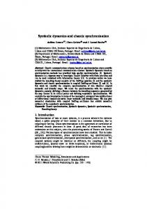
Figure 1: (a) Experimental time series of the laser intensity for a CO2 laser with feedback in the regime of homoclinic chaos. (b) Time expansion of a single orbit. (c) Phase space trajectory constructed by an embedding technique with appropriate delays (from Allaria et al. 2001).
An easy explanation of such a behavior is offered by the experimental results presented in Fig. 1, showing the alternation of large spikes and a small chaotic background. Rather than considering the time series
18
Arecchi
directly (Fig. 1a,b), it is convenient to construct the three dimensional (3D) trajectory in phase space by an embedding technique (Fig. 1c). For pedagogical reasons, we extract such a trajectory schematically in Fig. 2. Following the orbit, the phase point approaches the saddle focus S with a contraction rate α and then escapes from S with an expansion rate γ. In 3D the escape rate may be complex, γ + iα, providing oscillations. Whenever γ < α, we have so-called Shilnikov chaos (Arecchi et al. 1987), consisting of almost identical peaks P separated by a chaotic background. In that background, the proximity to the saddle focus S implies a large susceptibility, i.e. a large sensitivity to a forcing stimulus, thus making HC prone to lock to external signals. Some situations in which this locking is useful will be discussed in the next section.
Figure 2: Schematic view of the phase space trajectory approaching the saddle S and escaping from it. Chaos is due to the shorter or longer permanence around S. From a geometrical point of view, most of the orbit P provides regular spikes. For further details see text.
Thus, the first important point of this paper is that an array of weakly coupled HC systems represents a simple model for a physical realization of feature binding. Various experiments (Libet et al. 1979, Rodriguez et al. 1999) provide evidence that a perceptual decision is made after
Quantum Aspects of Chaotic Neuron Dynamics
19
T¯ ≈ 200 ms of exposure to a sensory stimulus. As we will elaborate in Sec. 5, synchronizing over 200 ms trains of spikes with a minimal interspike separation of 3 ms and an average spike rate of 25 ms corresponds to a repertoire of about 1011 different objects. T¯ ≈ 200 ms seems to be the time necessary to localize an element in the set of 1011 potential sensations and, hence, initiate some action. If a transient stimulus is presented for a time ∆T < T¯, then an uncertainty ∆P occurs in the set of all possible perceptions P . The second key point is the utilization of the synchronization pattern. Assume that a sensory layer (visual, auditory, etc.) receives two or more different stimuli as it is the case for ambiguous stimuli. Very early, the Gestalt psychologists measured the subjective response of individuals which includes the roughly periodic transition from one to the other perception. For instance, in the case of exposure to the Necker cube, a normal human individual switches from one perspective to the other, with a switching time in the range of a few seconds. It is pointless to recur to a hypothetical “homunculus” residing in the brain, reading the synchronization state of the sensory layers and acting accordingly, initiating motor actions such as escaping from a predator, catching a prey, or expressing linguistic utterances about sensations. As a viable alternative, we propose a simple model based on known brain components, consisting of coding neurons as described above and a reading system which localizes the boundaries of the synchronized domains and decides which is the prominent one based on a “majority rule”. As we will discuss in Sec. 6, the appropriate algorithm for extracting the time code is provided by a particular function which Wigner (1932) introduced in quantum mechanics. The Wigner algorithm consists in comparing a signal with a shifted version of itself and summing over all shifts with a phase factor introducing a Fourier transform (see also Mallat 1999). The time code is activated by the largest synchronized pattern established on the sensory layer. If there are different stimuli, the time coding must be preceded by a space coding which evaluates which one is the winning signal. This space coding is also reasonably performed by a Wigner function in space. Based on these considerations, we introduce a fundamental aspect of percept formation, namely, a quantum limitation in information encoding and decoding through spike trains, whenever the processing session is interrupted. In fact, the temporal coding requires a sufficiently long sequence of synchronized spikes in order to realize a specific percept. If the sequence is interrupted by the arrival of new uncorrelated stimuli, then an uncertainty ∆P emerges in the percept space P . This is related to the finite duration ∆T allotted for the code processing by the uncertainty relation ∆P · ∆T ≥ C
20
Arecchi
where C is a constant representing a quantum constraint on the coding. This means that the percepts are not set-theoretical objects, i.e. objects belonging to separate domains, but there are overlapping regions between them where it is impossible to discriminate one percept from another. In order to establish the above uncertainty relation we must introduce a metric and, hence, a distance in percept space. Furthermore we must consider whether for two different percepts separated by ∆P and observed for a duration ∆T the above relation is just the trivial overlap of two fuzzy sets, or whether it discloses a fundamental quantum feature implying interference. In the latter case, we propose to consider Wigner distributions to realize the decoding. They introduce appropriate phases which make the overlap wavelike. In conclusion, the subsequent sections will elaborate the following three main points: • Chaos, precisely homoclinic chaos, provides an efficient time code for classifying different percepts. • The code is read via a Wigner distribution; this provides quantum interference in the overlap region of different percepts. • The physiological decision time T¯ ≈ 200 msec is related to the lifetime of the interference; it corresponds to the decoherence time in quantum mechanics (Omn`es 1994, Zurek 1991). Quantum effects are expected when the perceptual task is truncated to ∆T < T¯.
2. Synchronization of Homoclinic Chaos A wide class of sensory neurons shows homoclinic chaotic spiking activity (Izhkievich 2000). More precisely, a saddle focus instability separates, in parameter space, an excitable region where axons are silent from a periodic region where the spike train is periodic (equal inter-spike intervals). If a control parameter is tuned at the saddle focus, the corresponding dynamical behavior (homoclinic chaos) consists of a frequent return to the unstable point (Allaria et al. 2001). This manifests itself as a train of identical spikes occurring, however, at erratic times (“chaotic” inter-spike intervals). Around the saddle focus the system displays a large susceptibility to external stimuli, hence it is easily adjustable and prone to respond to an input, provided it is composed of sufficiently low frequencies. (This means that such a system is robust against high frequency noise.) Such a type of dynamics has recently been explored in a series of reports that are here recapitulated as the following chain of linked facts.
Quantum Aspects of Chaotic Neuron Dynamics
21
1. A single spike in a 3D dynamics corresponds to a quasi-homoclinic trajectory around a saddle focus SF (fixed point with 1 (2) stable direction and 2 (1) unstable ones). The trajectory leaves the saddle and returns to it (Figs. 1,2). This behavior is called “quasihomoclinic” because, in order to stabilize the trajectory away from SF, a second fixed point, namely a saddle node SN, is necessary to assure a heteroclinic connection. 2. The homoclinic chaos (HC) shown in Figs. 1 and 2 has a localized chaotic tangle surrounded by an island of stability (Fig. 3, left). This provides a sensitivity region corresponding to the chaotic tangle and an active region corresponding to the identical spikes. Such a behavior is crucial to couple large arrays of HC systems, as it occurs in the coupling of neurons in the brain (Arecchi 2003). On the contrary, standard (e.g., Lorenz) chaos, where the chaotic behavior fills the whole attractor, is inconvenient for synchronization purposes (Fig. 3, right). 3. A train of spikes corresponds to the sequential return to, and escape from, the SF. A control parameter can be set at a value BC for which this return is erratic (“chaotic” inter-spike intervals) even though there is a finite average frequency. As the control parameter is set above or below BC , the behavior of the system moves from excitable (single spike triggered by an input signal) to periodic (regular sequence of spikes without input), with a frequency monotonically increasing with the separation ∆B from BC (Fig. 4). A low-frequency modulation of B around BC provides an alternation of silent intervals with periodic bursts. Such bursting behavior, typical of neurons in central pattern generators as the cardio-respiratory system, has been modeled by a laser experiment (Meucci et al. 2002). 4. Around SF, any tiny disturbance provides a large response. Thus, the homoclinic spike trains can be synchronized by a periodic sequence of small disturbances (Fig. 5). However, each disturbance has to be applied for a minimal time, below which it is not yet effective. This means that the system is insensitive to high-frequency noise (Zhou et al. 2003). 5. The above considerations prepare the ground for utilizing mutual synchronization as a convenient way to let different neurons respond coherently to the same stimulus, organizing themselves as a space pattern. A single dynamical system can be fed back by its own delayed signal (delayed self synchronization). If the delay is long enough, the system is decorrelated from itself, which is equivalent to feeding an independent system. This process allows to store
22
Arecchi
Figure 3: Comparison between HC (homoclinic chaos) (left column) and Lorenz chaos (right column). The top row is a phase space projection over two dynamical variables; SF denotes the saddle focus and SN the saddle node. On the left the two SF map onto each other after an inversion (x → −x, y → −y) with respect to the origin. The middle row shows the time series for variables x1 of HC (representing the laser intensity in the case of the CO2 laser) and x of Lorenz chaos. In the former case, a suitable threshold cuts on the chaotic background; in the latter case, no convenient region for thresholding can be isolated. Bottom row, left: after threshold, the new variable S(t) shows spikes alternating with flat regions where the system has a high sensitivity and short refractive windows where the intensity S(t) goes to zero.
Quantum Aspects of Chaotic Neuron Dynamics
23
Figure 4: Stepwise increase a) and decrease b) of a control parameter Bo by ±1% brings the system from homoclinic to periodic or excitable behavior. c) In case a) the frequency cr of the spikes increases monotonically with ∆Bo (from Meucci et al. 2002).
meaningful sequences of spikes as necessary for a short term memory (Arecchi et al. 2002). 6. A sketch of the dynamics of a single neuron is presented in Fig. 6; its HC behavior is discussed, e.g., by Izkhievich (2000). The feature binding conjecture, based on synchronization of different neurons exposed to the same image, is shown in Fig. 7 (Singer and Gray 1995). The role of threshold resetting due to past memories, as expressed in ART (Grossberg 1995), is illustrated in Fig. 8.
24
Arecchi
Figure 5: Experimental time series for different synchronization induced by periodic changes of the control parameter. (a) 1:1 locking, (b) 1:2, (c) 1:3, (d) 2:1 (from Allaria et al. 2001).
7. In the presence of stimuli localized over a few neurons, the corresponding disturbances propagate by inter-neuron coupling (either excitatory or inhibitory). A synchronized pattern is uniquely associated with each stimulus, different patterns compete. We conjecture that the resulting sensory response, which then triggers motor actions, corresponds by a majority rule to that pattern which has extended over the largest cortical domain. An example is discussed for two inputs to a one-dimensional array of coupled HC systems (Leyva et al. 2003).
Quantum Aspects of Chaotic Neuron Dynamics
25
Figure 6: Dynamical behavior of a single neuron. The sum of the inputs compares with a threshold level. If it is below (a) only a few noisy spikes occur as electrical activity on the axon; if it is just above (b) we have a periodic spike train, whose frequency increases as the input goes high above threshold (c).
These results have been established experimentally and confirmed by a dynamical model in the case of a class B laser2 with a feedback loop that readjusts the amount of losses depending on the value of the light intensity output (Arecchi et al. 1987). The facts listed above hold in general for any dynamical system which has a 3-dimensional sub-manifold separating a region of excitability from a region of periodic oscillations. Indeed, this “separatrix” has to be a saddle focus. In particular, all biological clocks are of HC type in order to have an adaptive period which can be re-adjusted whenever necessary (think, e.g., of the cardiac pace-maker).
3. Perceptions, Feature Binding, and Qualia Let us now return to the visual system, where the role of elementary feature detectors has been extensively studied in the past decades (Hubel 2 Class A lasers are ruled by a single order parameter, the amplitude of the laser field, which obeys a closed dynamical equation; all the other variables have a much faster decay rate, thus adjusting almost instantly to the local field value. Class B lasers are ruled by two order parameters, the laser field and the material energy storage providing the gain; the two degrees of freedom have comparable characteristic times and behave like a pair of activators and inhibitors in chemical dynamics (Arecchi 1987).
26
Arecchi
Figure 7: Feature binding: the lady and the cat are represented by the mosaic of empty and filled circles, respectively, each one representing the receptive field of a group of neurons in the visual cortex. Within each circle the processing refers to a specific detail (e.g. contour orientation). The relations between details are coded by the temporal correlations among neurons, as shown by the same sequences of electrical pulses for two filled circles or two empty circles. Neurons referring to the same individual (e.g. the cat) have synchronous discharges, whereas their spikes are uncorrelated with those referring to another individual (the lady) (from Singer and Gray 1995).
1995). By now we know that some neurons are specialized in detecting exclusively vertical or horizontal bars, or a specific luminance contrast, etc. However, the problem of how elementary detectors contribute to a holistic (Gestalt) perception is still unsolved. Singer and Gray (1995) provide a hint: Suppose we are exposed to a visual field containing two separate objects. Both objects are made of the same visual elements, horizontal and vertical contours, different degrees of luminance, etc. What are then the neural correlates of the identification of the two objects? We have one million fibers connecting the retina to the visual cortex. Each fiber results from the merging of approximately 100 retinal detectors (rods and cones) and, as a result, it has its own receptive field. Each receptive field isolates a specific detail of an object (e.g. a vertical bar). We thus split an image into a mosaic of adjacent receptive fields. The well-known “feature binding” hypothesis assumes that all those cortical neurons, whose receptive fields are hit by a specific object, synchronize their spikes and, as a consequence, the visual cortex organizes
Quantum Aspects of Chaotic Neuron Dynamics
27
Figure 8: Adaptive resonance theory. Role of bottom-up stimuli from the early visual stages and top-down signals due to expectations formulated by the semantic memory. The focal attention assures the matching (resonance) between the two streams (from Julesz 1991).
into separate neuron groups defined by synchronization. Direct experimental evidence of this synchronization is obtained by inserting microelectrodes into the cortical tissue of animals and sensing multiple single neurons (Fig. 7; Singer and Gray 1995). Indirect evidence of synchronization based on EEG data has been obtained for human beings as well (Rodriguez et al. 1999). The advantage of such a temporal coding scheme as compared to rate-based codes, which rely on the pulse rate averaged over a time interval and which have been exploited in communication engineering, has been discussed recently (Softky 1995). Based on the neurodynamical results reported above, we can understand more details of feature binding (Grossberg 1995). The higher cortical stages, where synchronization takes place, have two inputs. One (bottom-up) comes from the sensory detectors via the early stages which classify elementary features. This single input is insufficient, because it would provide the same signal for, e.g., horizontal bars belonging indifferently to either one of the two objects. However, as already mentioned, each neuron is a nonlinear system passing close to a saddle point. The application of a suitable perturbation can stretch or shrink the interval of time spent around the saddle, and thus lengthen or shorten the inter-spike interval. The perturbation consists of top-down signals corresponding to conjectures made by the semantic memory (Fig. 8). In other words, the perception process is not like the passive imprinting of a camera film, but it is an active process whereby external stimuli
28
Arecchi
are interpreted in terms of past memories. A focal attention mechanism assures that a matching is eventually reached. This matching consists of resonant or coherent behavior between bottom-up and top-down signals. If matching does not occur, different memories are tried, until the matching is realized. In the presence of a fully new image without memorized correlates, the brain has to accept the fact that it is exposed to a new experience. Notice the advantage of this time dependent use of neurons, which become available to be active in different perceptions at different times, as compared to the paradigm of fixed memory elements, which store a specific object and are not available for others (the so-called “grandmother neuron” hypothesis). We have above presented qualitative reasons why the degree of synchronization represents the perceptual salience of an object. Synchronization of neurons located even at large distances from each other yields a space pattern in the sensory cortex, which can extend over a few square millimeters, involving millions of neurons. The winning pattern is determined by dynamic competition (the so-called “winner takes all” dynamics). Perceptual knowledge appears as a complex self-organizing process. Naively, one might expect that a given “quale”, i.e. a private sensation as, for instance, the red of a Tizian painting, is always coded by the same sequence of spikes. If so, in the near future of such a sensation the corresponding information could be retrieved by a high resolution detector, and hence a Rosetta stone could be established relating particular spike sequences to particular qualia. Such a naive expectation would ultimately lead to a world without privacy, and is altogether wrong for the following reasons. After the initial formation of a quale, i.e. the first time of its experience, any further repetition of that experience, either by memory recollection or by re-perceiving the painting, occurs under new and different circumstances (one has become older, memory storage has drastically mutated). These novelties imply that feature binding is realized by a modified synchronization pattern. Corresponding evidence has been established by Freeman’s (1991) research on the synchronization pattern of the olfactory bulb in rabbits, recorded using a large number of electrodes. As the same odor is presented twice, with an intermediate odor in between, the two synchronization patterns are altogether different, even though the animal behavior hints at the same reaction. The distinction between stimulus-induced and ongoing brain activity is more clearly established by real-time optical imaging (Arieli et al. 1996). Freeman’s results are contrasted by the fact that some olfactory neurons of the locust yield the same bursts of spikes for the same odor (Rabinovich et al. 2001). Presumably, lower animals such as locusts have a much smaller semantic repertoire than rabbits or humans. For this reason, their behavior may be a little less far away from the concept of the Rosetta stone.
Quantum Aspects of Chaotic Neuron Dynamics
29
4. A Metric in Percept Space In order to study different percepts in terms of their distance ∆P in percept space, and then establish the uncertainty relation indicated in Sec. 1, a convenient metric space for percepts must be introduced. A metric D is essentially an abstract distance. By definition, metrics have the following properties: • D(Sa , Sa ) = 0 • Symmetry: D(Sa , Sb ) = D(Sb , Sa ) • Triangle inequality: D(Sa , Sc ) ≤ (D(Sa , Sb ) + D(Sb , Sc ) • Non-negativity: D(Sa , Sb ) > 0 unless Sa = Sb We discuss two proposals for a metric of spike trains. The first one, by Victor and Purpura (1997), considers each spike as very short and each coincidence as an instantaneous event with no time uncertainty. The metric spans a large, yet discrete space and can be evaluated using standard computers. A more recent proposal by Rossum (2001) accounts for the physical fact that each spike is spread in time by a filtering process. Hence overlaps between two spikes have a time width tc and any coincidence is a smooth continuous process. Indeed, as discussed above, in neurodynamics the high-sensitivity region around the saddle focus has a finite width in time. While the discrete metric allows a set-theoretical interpretation, the continuous metric fits better with neurodynamical facts. Victor and Purpura (1997) introduced several families of metrics between spike trains as a tool to study the nature and precision of temporal coding. Each metric defines the distance between two spike trains as the minimal “cost” required to transform one spike train into the other via a sequence of allowed elementary steps, such as inserting or deleting a spike, shifting a spike in time, or changing an inter-spike interval length. The geometries corresponding to these metrics are in general not Euclidean, and distinct families of cost-based metrics typically correspond to distinct topologies on the space of spike trains. Each metric, in essence, represents a candidate temporal code in which similar stimuli produce responses which are close and dissimilar stimuli produce responses which are distant. On this proposal, spike trains are considered as points in an abstract topological space. A spike train metric is a rule which assigns a nonnegative number D(Sa , Sb ) to pairs of spike trains Sa and Sb , which expresses how dissimilar they are. Successful applications have been reported by MacLeod at al. (1998). Rossum (2001) introduced an Euclidean distance measure computing the dissimilarity between two spike trains. First of all, one filters both
30
Arecchi
spike trains assigning a duration tc to each spike. In our language, this would be the time extension of the saddle point region of high susceptibility, where perturbations are effective. To calculate the distance between two spike trains, their integrated squared difference is evaluated. The simplicity of this distance measure enables an analytical treatment of simple cases. Numerical implementation is straightforward and fast. Rossum’s distance interpolates between, on the one hand, counting non-coincident spikes and, on the other hand, counting the squared difference in total spike count. In order to compare spike trains with different rates, total spike counts can be used (large tc ). However, for spike trains with similar rates, the difference in total spike number is not useful and coincidence detection is sensitive to noise. Rather than convolving the distance with an exponential kernel, as is usually done, one could alternatively convolve the spikes with a rectangular window. In that case the situation becomes somewhat similar to binning followed by calculating the Euclidean distance between the number of spikes in the bins. But in standard binning the bins are fixed on the time axis, therefore two different spike trains yield identical binning patterns as long as spikes fall into the same bin. However, with the proposed distance (convolving with either a rectangle or an exponential) this does not happen. The distance is zero only if the two spike trains are fully identical (assuming tc is finite). Since the continuous distance introduced here is explicitly embedded in Euclidean space, it is less general but easier to analyze than the discrete distance introduced by Victor and Purpura (1997). Interestingly, the distance is related to stimulus reconstruction techniques, where convolving the spike train with the spike-triggered average yields a first-order reconstruction of the stimulus (Rieke et al. 1996). Here the exponential corresponds roughly to the spike-triggered average, and the filtered spike trains correspond to the stimulus. The distance thus approximately measures the difference in the reconstructed stimuli. This might well explain the linearity of the measure for intermediate tc . The relevance of both discussed attempts to introduce a metric in percept space is limited due to the critical stance concerning qualia, which was outlined above. Indeed, due to the subjective introduction of new elements of experience, two spike trains referring to the same quale could be far away from each other in percept space. The simplistic stimulusresponse paradigm of behaviorism, which may work for lower animals such as locusts, fails for higher animals where qualia represent a richness which is sensitive to tiny differences of environmental features. The influence of the environment can induce “decoherence” between two perceptions corresponding to similar stimuli. For the remainder of the paper, we make the over-simplifying assumption (perhaps fully applicable only to invertebrates) that a percept space
Quantum Aspects of Chaotic Neuron Dynamics
31
is in one-to-one correspondence with a stimulus space. This will allow us to develop our arguments in a relatively uncomplicated way and to propose persuasive quantum considerations.
5. The Role of Duration T¯ in Perception: A Quantum Aspect How does a synchronized pattern of neuronal activity potentials become a relevant perception? This is an active area of investigation which may be split into many hierarchical levels. Notice however that, due to the above consideration of qualia, the experiments discussed in this section hold for purely a-semantic perceptions only. This is to say that we restrict ourselves to the detection of rather elementary features which would not trigger any categorization skills. Not only the different receptive fields of the visual system, but also of other sensory channels as auditory, olfactory etc. integrate individual stimuli into a holistic perception via feature binding. Its meaning is “decided” in the pre-frontal cortex (PFC), which represents a kind of arrival station from the sensory areas and a point of departure for signals going to the motor areas. On the basis of the perceived information, motor actions are started, including linguistic utterances (Rodriguez et al. 1999). Sticking to the neurodynamical level, and leaving the investigation of higher levels of organization to psychophysics, we stress here a fundamental temporal limitation. Taking into account that each spike lasts about 1 msec, that the minimal inter-spike separation is 3 msec, and that the decision time at the PFC is estimated as T¯ ≈ 200 msec, we can split T¯ into 200/3 = 66.6 bins of 3 msec duration, which are designated by 1 or 0 depending on whether they contain a spike or not. Thus, there is a total number of 266 ≈ 6 × 10¹⁹ different messages which can be transmitted. However, we must also account for the average rate at which spikes proceed in our brain (r = 40 Hz, average ISI = 25 msec). Accounting for this rate, we can evaluate a reduction factor α = S/T¯ = 0.54 where S is an entropy (Strong et al. 1998, MacKay and McCulloch 1952), thus there are roughly 2S = 1011 words with significant probability. Even though this number is large, we are still within a finite realm. Provided we had time enough to ascertain which one of the different messages we are dealing with, we could classify it with the accuracy of a digital processor, without residual error. But suppose we expose the cognitive agent to fast changing scenarios, for instance by presenting sequences of unrelated video frames with a time separation less than 100 msec. While small gradual changes induce the sense of motion such as in movies, big differences imply completely different subsequent spike trains. Here, any spike train gets interrupted
32
Arecchi
after a duration ∆T less than the canonical T¯. This means that the brain cannot decide among all coded perceptions which share the same structure up to ∆T but are different afterwards. Whenever we stop the perceptual task at a time ∆T shorter than the total time T , then the bin stretch T − δT (from now on we refer to time in units of bins) is not explored. This means that all stimuli providing equal spike sequences up to ∆T and differing afterwards will cover an uncertainty region ∆P whose size is given by ∆P = 2αT 2−α∆T = PM e−α∆T ln2
(1)
where PM ≈ 1011 is the maximum perceptual size available with the chosen T¯ ≈ 66.6 bins per perceptual session and rate ν = 40 Hz. Relation (1) is very different from the standard uncertainty relation ∆P · ∆T ≥ C
(2)
that we would expect in a word-bin space ruled by Fourier transform relations. Indeed, the transcendental equation (1) is more rapidly converging at short and long ∆T than the hyperbolic relation (2). We fit (1) by (2) in the neighborhood of a small uncertainty ∆P = 10 words, which corresponds to ∆T = 62 bins. Around ∆T = 62 bins the local uncertainty (2) yields a constant C = 10 · 62 = 620 words × bins As an example, let us consider two nearby musical tones at 440 Hz (A or la) and 480 Hz (B or si), respectively, i.e. 1.32 and 1.44 periods/bin. After an observation time of ∆T = 62 bins the numbers of perceived periods are 81.84 and 89.29, respectively, yielding a square separation D2 = (7.44)2 = 55.35 Normalizing D2 with respect to C, we obtain the separation in word-bin space of the two sound percepts limited at ∆T , i.e. D2 55.35 = �1 C 620 We thus expect that the decoherence time between the superposition of the two tones is reduced with respect to the standard perception time by a factor which is much less than 1. Thus we expect strong interference, at variance with the transition from microscopic to mesoscopic physics where the reduction denominator is usually dramatically bigger than 1, namely of the order of D2 /�. The problem faced so far in the scientific literature, that of an abstract comparison of two spike trains without accounting for the available time
Quantum Aspects of Chaotic Neuron Dynamics
33
for such a comparison, is rather unrealistic. A finite available time ∆T plays a crucial role in any decision, either for identifying an object within a fast sequence of different perceptions or for retrieving memorized patterns in order to decide about an action. As a result, the perceptual space P per se is meaningless. What is relevant for cognition is the joint (P, T ) space, since in vivo there is always a limited time ∆T which may truncate the whole spike sequence upon which a given perception has been coded. Only in vitro we allot to each perception all the time necessary to classify it. Let us consider the following thought experiment. Take two percepts P1 and P2 which for long processing times appear as the two stable states of a bistable optical illusion, e.g. the Necker cube. If we restrict the observation time to ∆T , then the two uncertainty areas overlap. The contours drawn in Fig. 9 show this qualitatively.
Figure 9: Uncertainty areas of two perceptions P1 and P2 for two different spike trains. In the case of short ∆T , the overlap region is represented by a Wigner function with strong positive and negative oscillations which T along the T axis. The frequency is given by the ratio evolve as cos ∆P C of the percept separation ∆P = P2 − P1 with respect to the perceptual constant C.
This situation is similar to the non-commutative position-momentum space of a single quantum particle. In this case, the quasiprobability Wigner function has strong non-classical oscillations in the overlap region (Zurek 1991). We cannot split the position-momentum space into two disjoint domains (sets) to which a Boolean logic or a classical Kolmogorov probability is applicable. This is the reason why Bell’s inequalities are violated in experiments dealing with such a situation (Omn`es 1994).
34
Arecchi
The Wigner function formalism derives from a Schr¨ odinger wavefunction treatment for a pure state and a corresponding density matrix for mixed states. In the perceptual (P, T ) space, no Schr¨odinger treatment is available, but we can apply a reverse logical path as follows. Due to the uncertainty relation ∆P ∆T ≥ C, a partition of the (P, T ) space into sets is inadmissible if the (P, T ) space is non-commutative. Thus it must be susceptible to a Wigner function treatment, and we can consider the contours of Fig. 9 as fully equivalent to isolevel cuts of a Wigner function. Hence we can interpret the interference of distinct states analogous to quantum physics. This means that in neurophysics time occurs in two completely different meanings. One of them is the ordering parameter used to describe the succession of events, and the other is the duration of a relevant spike sequence, i.e. of a synchronized train. On the second meaning, time T is a variable conjugate to perception P . The quantum aspect of perception emerges as a necessity from the analysis of an interrupted spike train in a perceptual process. It follows that the (P, T ) space cannot be partitioned into disjoint sets to which a Boolean yes/no relation is applicable. Hence, ensembles cannot obey classical probabilities. A set-theoretical partition, however, is the prerequisite to apply the Church-Turing theorem, which establishes the equivalence of recursive functions on a set and operations of a universal computer. Therefore, the derived arguments for interfering perceptions should rule out in principle a finite character of perceptual processes. This would provide a negative answer to Turing’s question of whether mental processes can be simulated by a universal computer (Turing 1950). Quantum limitations were also proposed by Penrose (1994), but on a completely different basis. In his proposal, the quantum character was attributed to the physical behavior of “microtubuli”, microscopic components of neurons playing a central role in synaptic activity. However, speaking of quantum coherence at the quantum level in biological processes is implausible if one accounts for the extreme vulnerability of any quantum system to decoherence processes. These make quantum superposition effects observable only in extremely controlled laboratory situations and at sub-picosecond time scales that are not relevant for synchronization in the 10–100 msec range. Nevertheless, biologically interesting decoherence time scales, e.g. for microtubuli, remain a topic of hot discussion (Tegmark 2000, Hagan et al. 2002). Our tenet is that the quantum level in a living being emerges from the limited time available in order to make vital decisions. It is logically based on a non-commutative set of relevant variables and, hence, requires the logical machinery of the traditional quantum description of the microscopic world, where non-commutativity results from the use of variables such as positions and momenta. Contemporary discussions (Omn`es 1994)
Quantum Aspects of Chaotic Neuron Dynamics
35
have clearly excluded the need for hidden variables and the possibility that the quantum formalism could be a projection of a more general classical approach. Similarly, in our case, the fact that decisions are made on the basis of, say, a 200 msec sequence of neuronal spikes excludes a cognitive world in which longer decision times (say, 400 msec) would disentangle overlapping states. In other words, the universe of perceptual 200 msec events would be correctly described by a “cognitive” quantum formalism, since perceptual facts would be considered inaccessible at the time scale of 400 msec. The qualitative uncertainty considerations have been addressed as “quantum” by postulating an interference within the overlapping region. More precisely, if we have a sequence of identical spikes of unit area localized at erratic time positions τ1 , then the whole sequence is represented by � f (t) = δ(t − τl ) (3) l
where {τl } is the set of positions of the spikes. A temporal code, based on the temporal structure of spike trains, depends on the moments of the distributions of inter-spike intervals (ISI)l = {τl − τl−1 } .
(4)
Different ISIs encode different sensory information. A time ordering within the sequence (3) is established by comparing the overlap of two signals as (3) is mutually shifted in time. Weighting all shifts with a phase factor and summing up, this amounts to constructing a Wigner function (cf. Wigner 1932, Mallat 1999): � +∞ W (t, ω) = f (t + τ /2) f (t − τ /2) exp(iωτ ) dτ (5) −∞
If f is the sum of two spike trains f = f1 + f2 as in Fig. 10, the frequencytime plot displays an intermediate interference. Eq. (5) provides interference whatever the time separation between f1 and f2 is. In fact, we know that the decision time T¯ truncates a perceptual task, thus we must introduce a cutoff function g(τ ) = exp(−τ 2 /T¯2 ) which transforms the Wigner function as � +∞ W (t, ω) = f (t + τ /2) f (t − τ /2) exp(iωτ ) g(τ ) dτ
(6)
(7)
−∞
Using quantum terminology, the brain physiology breaks the quantum interference for t > T¯ due to decoherence (Omn`es 1994).
36
Arecchi
Figure 10: Wigner distribution of two localized sinusoidal packets shown at the top. The oscillating interference is centered at the middle timefrequency location (from Mallat 1999).
6. Who Reads the Information Encoded in a Synchronized Neuron Array? The Role of the Wigner Function We have seen that feature binding in perceptual tasks implies the mutual synchronization of axonal spike trains in neurons which can be even far away and yet contribute to a well defined perception by sharing the same pattern in a spike sequence. The synchronization conjecture, put forward, e.g., by von der Malsburg (1981), was later given direct experimental evidence by inserting several micro-electrodes probing neurons in the cortex of cats and then studying the temporal correlation in their responses to specific visual inputs (Singer and Gray 1995). For human brains, indirect evidence for synchronization was acquired by exposing a subject to transient patterns and recording time-frequency plots of the EEG signals (Rodriguez et al. 1999). Even though the spatial resolution is poor, significant phase correlations among EEG signals from different cerebral areas at different times were reported. Recently, the dynamics of HC has been explored in some mathematical aspects which display strong analogies with the dynamics of biological clocks, in particular that of model neurons (Hodgkin and Huxley 1952, Izhikevich 2000). HC provides almost equal spikes occurring at variable time positions and presents a region of high sensitivity to external stimuli. Perturbations arriving within the sensitivity region can easily induce synchronization, either to an external stimulus or to other HC neurons (mutual synchronization) within a coupled array.
Quantum Aspects of Chaotic Neuron Dynamics
37
In view of the above facts, we can model the encoding of external information in a sensory cortical area (e.g. V1 in the case of vision) as a particular spike train assumed by an input neuron directly exposed to the arriving signal and then propagated through the network. As shown by series of experiments on feature binding (cf. Singer and Gray 1995), we must transform the local time information provided by Eqs. (3) and (4) into a spatial information describing the degree to which a cortical area is synchronized. If many sites are synchronized by mutual coupling, then the read-out problem consists in tracking the pattern of values (3), one for each site. Let us take for simplicity a continuous site index x. In the case of two or more different signals applied at different sites, competition starts and we conjecture that the winning information (that is, the one which is then passed on to a decision center and becomes enacted) corresponds to a “majority rule”. For example, if the encoding layer is a 1-dimensional chain of N coupled sites activated by external stimuli at the two ends (i = 1 and i = N ), the majority rule says that the prevailing signal is that which has synchronized more sites. The crucial question is then: who reads that information in order to decide upon? As already mentioned above, we cannot recur to some homunculus who reads the synchronization state. Indeed, because it is realized by physical components, the homunculus itself would require a reading neuron layer, followed by some interpreter which would be a higher level homunculus, and so on, implying a “regress ad infinitum”. On the other hand, it is well known that, as we map the interconnections in the visual system, V1 projects through the ventral stream and the dorsal stream toward the inferotemporal cortex and the parietal cortex, respectively. The two streams contain a series of intermediate modules characterized by receptive fields of increasing size. To show how this cascade of modules can localize the interface between two domains corresponding to different synchronizations, we start with the result that simple cells with center-surround organization of receptive fields (Hubel 1995) perform first- and second-order spatial derivatives. Suppose this operation was done in a particular module. At the successive module, as the converging process moves, two second derivative signals will converge on a simple cell which then perform a higher-order derivative, and so on. In this way, we build a power series of spatial derivatives. A translated function such as f (x+ξ) is then reconstructed by stacking many modules, as can be checked by a Taylor expansion. For symmetric situations, the contributions of odd derivatives cancel each other.3 3 Note that the alternative of exploring different neighborhoods ξ of x by varying ξ would imply a moving pointer to be set sequentially at different positions. There is no correspondence for this in brain physiology.
38
Arecchi
The next step consists in comparing the function f (x + ξ) with a suitable standard to evaluate it. Since there are no such standards embedded in a living brain, this procedure must be done by comparing f with a shifted version of itself, something like the product f (x + ξ)f (x − ξ). Such a product can be naturally performed by letting the two signals f (x ± ξ) converge onto the same neuron, exploiting the response characteristic limited to the lowest quadratic nonlinearity, by taking the square of the sum of the two converging inputs and isolating the product. This operation is completed by summing up the different contributions corresponding to different values of ξ, with a kernel that keeps track of the scanning over different ξ, preserving information about different domain sizes. If this kernel was just a constant, we would obtain a trivial average which cancels the information about ξ. With no loss of generality, we adopt a Fourier kernel exp(ikξ), effectively leading to +∞ �
f (x − ξ) f (x + ξ) exp(ikξ) dξ
W (x, k) =
(8)
−∞
W (x, k) is thus a Fourier transform with respect to ξ, called Wigner-Ville function. It contains information about both the position x, around which local behavior is explored, and the frequency k associated with the spatial resolution. As it is well known from quantum mechanics or electrical engineering, where this function is currently used, it contains the maximally available information compatible with the Fourier uncertainty ∆x∆k ≥ 1
(9)
Such an intrinsic limitation is implied by any joint extraction of information about position (x) and resolution (k) by physical measuring operations. In summary, it appears that the Wigner function represents the best read-out strategy of a synchronized module that can be done by exploiting natural machinery rather than recurring to a homunculus. The local value of the Wigner function represents a decision signal to be sent to motor areas triggering suitable action. Now, let us explore the appropriate function f (x) whose space pattern represents the relevant information stored in a sensory module. The pending problem is how to bring space and time information together. When many sites are coupled, there is a fixed time lag t∗ between the occurrence of spikes at adjacent sites. Even without accounting for axonal transmission, a delay is introduced by the fact that input from a previous site is sensed only when the driven system is within the saddle focus region. This implies a site-to-site delay, whose value depends on whether
Quantum Aspects of Chaotic Neuron Dynamics
39
the coupling is positive or negative. In the presence of a single input, the overall synchronization needs a time N t∗ , N being the site order. This corresponds to a velocity 1 v= ∗ (10) t to be measured in sites per second. The new feature, which is peculiar of the Wigner function construction, is the so-called “Schr¨ odinger cat paradox” in quantum mechanics. If we have established that physical measurements consist of building up a Wigner function, then we must accept that in addition to the two patches associated with a “living cat” and a “dead cat” there must be an oscillating interference as well. From 1935 to 1995 this has been considered a pseudo-philosophical problem; nowadays such an extra term for the interference can acquire significance if the superposition refers to states of microscopic objects as atoms or photons rather than cats. (Moreover, its existence is crucial for quantum computation.) The reason why we often do not see interference is decoherence. If the system under observation interacts with its environment, then the two states of the superposition have a finite lifetime. This so-called decoherence time, after which the interference vanishes, decreases with an increasing separation between the two states. While the separation is still manageable for the two polarization states of a photon, it is too large for the two states of a macroscopic quantum system. If we call τi the intrinsic decay time of each of the two states of the superposition, then the mutual interference in the Wigner function decays with the decoherence time τdec =
τi D2
(11)
where D2 is the square of the separation D in phase space between the centers of the Wigner functions of the two separate states. Notice that, in microscopic quantum physics, D2 is measured in units of Planck’s action �. Usually D2 /� is much greater than one for a macroscopic system and hence the observation time is too long to detect a coherent superposition. Instead, in neurodynamics, we perform measurement operations which are limited by the intrinsic space and time resolutions typical of brain processes. The associated uncertainty constant C is such that it is very easy to have a relation such as (11) with D2 /C of the order of one, and hence superposition lifetimes comparable to time scales of standard neural processes. This substantiates the conjecture that for short times or close cortical domains a massive parallelism typical of quantum computation is possible. The threshold readjustment due to expectations arising from past memory acts as an environmental disturbance, which orthogonalizes different neural states, thus destroying parallelism.
40
Arecchi
7. Summary A central issue of cognitive neuroscience concerns the way in which a large collection of coupled neurons combines external signals with internal memories into new coherent patterns of meaning. Such a process is called “feature binding” insofar as the coherent patterns combine together features which are extracted separately by specialized cells, but which do not make sense as isolated items. A powerful conjecture, with experimental confirmation, is that feature binding in perceptual tasks implies the mutual synchronization of spike trains in neurons which can reside in distant neurons and yet contribute to a well-defined perception by sharing the same sequence. Based on recent laboratory investigations of homoclinic chaotic systems and their mutual synchronization by weak coupling, a novel conjecture on the dynamics of single neurons is formulated. Homoclinic chaos implies the recurrent return of the dynamical trajectory to a saddle focus, in whose neighbourhood the system susceptibility (response to an external perturbation) is very high, which makes it easy to lock to an external stimulus. Thus homoclinic chaos appears as a suitable way to encode information in time by trains of equal spikes occurring at apparently erratic times. A standard measurement consists in setting a meter’s pointer to a given number and then assigning to the measured object a position corresponding to the number displayed by the meter. On the other hand, a set assignment based on a synchronized sequence of spikes requires a decision time T¯ sufficiently longer than the minimal inter-spike separation t1 , so that the total number of different set elements is related in some way to T¯/t1 . Neuronal estimates for these quantities are T¯ ≈ 200 msec and t1 ≈ 3 msec. In a sensory layer of the neocortex an external stimulus localized at some input spreads over a large assembly of coupled neurons, building up a collective state univocally corresponding to the stimulus. Thus, the synchronization of spike trains of many individual neurons is the basis of a coherent perception. In order to classify the set of different perceptions, at least in principle, the percept space can be given a metric structure by introducing a distance measure. The distance in percept space is conjugate to the duration of the perceptual process in the sense that an uncertainty relation in percept space is associated with time-limited perceptions. This coding of different percepts by synchronized trains of spikes entails fundamental quantum features. If the synchronized spike trains are truncated at a time ∆T < T¯, then the corresponding identification of a percept P is not fully accomplished, but carries an uncertainty cloud ∆P around P . As two uncertainty clouds around two distinct percepts overlap, interference occurs as a typical quantum phenomenon.
Quantum Aspects of Chaotic Neuron Dynamics
41
It is conjectured that the corresponding quantum formalism is not exclusively restricted to microscopic phenomena but represents the appropriate description of truncated perceptions. The explored quantum feature is uniquely tied up to the coding and reading operations which take place in passing from external signals on the sensor transducers to complete perceptions driving an action. It is not related to Planck’s action but to the details of the perceptual chain.
References Allaria E., Arecchi F.T., Di Garbo A., Meucci R. (2001): Synchronization of homoclinic chaos. Physical Review Letters 86, 791–794. Arecchi F.T. (1987): Instabilities and chaos in single mode homogeneous line lasers. In Instabilities and Chaos in Quantum Optics, ed. by F.T. Arecchi and R.G. Harrison, Springer, Berlin, pp. 9–48. Arecchi F.T., Meucci R., Gadomski W. (1987): Laser dynamics with competing instabilities. Physical Review Letters 58, 2205–2208. Arecchi F.T. (2000): Complexity and adaptation: a strategy common to scientific modeling and perception. Cognitive Processing 1, 23–34. Arecchi F.T., Meucci R., Allaria E., Di Garbo A., Tsimring L.S. (2002): Delayed self-synchronization in homoclinic chaos. Physical Review E 65, 046237. Arecchi F.T., Allaria E., Leyva I. (2003): A propensity criterion for networking in an array of coupled chaotic systems. Physical Review Letters, accepted for publication. Arieli A., Sterkin A., Grinvald A., Aertsen A. (1996): Dynamics of ongoing activity: explanation of the large variability in evoked cortical responses. Science 273, 1868–1871. Edelman G.M. and Tononi G. (1995): Neural Darwinism: The brain as a selectional system. In Nature’s Imagination: The Frontiers of Scientific Vision, ed. by J. Cornwell, Oxford University Press, New York, pp. 78–100. Freeman W.J. (1991): The physiology of perception. Scientific American 264(2), 78–85. Grossberg S. (1995): The attentive brain. American Scientist 83, 438–449. Hagan S., Hameroff S.R., and Tuszynski J.A. (2002): Quantum computation in brain microtubules: decoherence and biological feasibility. Physical Review E 65, 061901-1 bis -11. Hodgkin A.L. and Huxley A.F. (1952): A quantitative description of membrane current and its application to conduction and excitation in nerve. Journal of Physiology 117, 500–544. Hubel D.H. (1995): Eye, Brain, and Vision. W.H. Freeman, New York. Izhikevich E.M. (2000): Neural excitability, spiking, and bursting. International Journal of Bifurcation and Chaos 10, 1171–1266.
42
Arecchi
Julesz B. (1991): Early vision and focal attention. Reviews of Modern Physics 63, 735–772. Leggett A.J. and Garg A. (1985): Quantum mechanics versus macroscopic realism: is the flux there when nobody looks? Physical Review Letters 54, 857–860. Leyva I., Allaria E., Boccaletti S., Arecchi F.T. (2003): Competition of synchronization patterns in arrays of homoclinic chaotic systems. Physical Review E, accepted for publication. Libet B., Wright E.W., Feinstein B., Pearl, D.K. (1979): Subjective referral of the timing for a conscious sensory experience. Brain 102, 193–224. MacKay D. and McCulloch W.S. (1952): The limiting information capacity of neuronal link. Bulletin of Mathematical Biophysics 14, 127–135. MacLeod K., Backer A., Laurent G. (1998): Who reads temporal information contained across synchronized and oscillatory spike trains? Nature 395, 693– 698. Mallat S. (1999): A Wavelet Tour of Signal Processing, Academic Press, San Diego. Malsburg von der C. (1981): The correlation theory of brain function. Internal Report 81-2, Max-Planck-Institut f¨ ur biophysikalische Chemie, G¨ ottingen. Reprinted in Models of Neural Networks II, ed. by E. Domany, J.L. van Hemmen and K. Schulten, Springer, Berlin 1994, pp. 95–119. Meucci R., Di Garbo A., Allaria E., Arecchi F.T. (2002): Autonomous bursting in a homoclinic system. Physical Review Letters 88, 144101. Omn`es R. (1994): The Interpretation of Quantum Mechanics, Princeton University Press, Princeton. Penrose R. (1994): Shadows of the Mind, Oxford University Press, New York. Rabinovich M., Volkovskii A., Lecanda P., Huerta R., Abarbanel H., Laurent G. (2001): Dynamical encoding by networks of competing neuron groups. Physical Review Letters 87, 068102. Rieke F., Warland D., de Ruyter van Steveninck R., Bialek W. (1996): Spikes: Exploring the Neural Code, MIT Press, Cambridge Mass. Rodriguez E., George N., Lachaux J.P., Martinerie J., Renault B., Varela F. (1999): Perception’s shadow: long-distance synchronization in the human brain. Nature 397, 340–343. Rossum van M. (2001): A novel spike distance. Neural Computation 13, 751– 763. Singer W. and Gray C.M. (1995): Visual feature integration and the temporal correlation hypothesis. Annual Reviews of Neuroscience 18, 555–586. Softky W. (1995): Simple codes versus efficient codes. Current Opinions in Neurobiology 5, 239–247. Stapp H. (2001): Quantum theory and the role of mind in nature. Foundations of Physics 31, 1465–1499. Strong S.P., Koberle R., de Ruyter van Steveninck R., Bialek W. (1998): Entropy and information in neural spike trains. Physical Review Letters 80, 197– 200.
Quantum Aspects of Chaotic Neuron Dynamics
43
Tegmark M. (2000): The importance of quantum decoherence in brain processes. Physical Review E 61, 4194–4206. Turing A. (1950): Computing Machinery and Intelligence. Mind 59, 433–460. Ullman S. (1996): High-Level Vision, MIT Press, Cambridge Ma. Victor J.D. and Purpura K.P. (1997): Metric-space analysis of spike trains: theory, algorithms and application. Network: Computation in Neural Systems 8, 127–164. Vitiello G. (2000): My Double Unveiled: the Dissipative Quantum Model of Brain, Benjamin, Amsterdam. Wigner E.P. (1932): On the quantum correction for thermodynamic equilibrium. Physical Review 40, 749–759. Zhou C.S., Allaria E., Boccaletti S., Meucci R., Kurths J., Arecchi F.T. (2003): Noise induced synchronization and coherence resonance of homoclinic chaos. Physical Review E 67, 015205. Zurek W.H. (1991): Decoherence and the transition from quantum to classical. Physics Today (October), 36–44.
Received: 02 July 2003 Revised: 06 September 2003 Accepted: 01 October 2003 Reviewed by G¨ unter Mahler and Stefan Rotter.