International Journal of Mechanical Engineering and Research Volume 5 Issue 1 (Page, 7-14), ISSN: 2277-8128
Evaluation of Sound Power through Sound Intensity Technique Eliezer Pacheco1, Alfredo Calixto2, Wiliam Alves Barbosa3, Paulo Henrique Trombetta Zannin4 1, 2, 3, 4. Laboratory of Environmental and Industrial Acoustic and Acoustic Comfort – LAAICA, Department of Mechanical Engineering, Federal University of Paraná, Brazil, Corresponding author:
[email protected]
Abstract - This study was performed to evaluate the differences in noise level produced by an eccentric press, during the manufacturing of metallic closures for steel cans. The primary objective of the study was to establish a rank of sound intensity level and sound power level as well as the global noise level emitted by this particular press. Ten different areas in the surface surrounding the press were evaluated regarding both the sound power and the sound intensity of each measurement. Each site was measured twice to increase accuracy. The 10 areas sampled were sweeping using intensity’s probe. We have found the surface area to demonstrate the lowest noise level was at S1 and the highest one was at S10. In conclusion, our study demonstrates adequately the global noise level as well as in specific sites, indicating area requiring special treatment for noise reduction in this environment. Keywords: sound intensity, sound power,
1. INTRODUCTION Often an application of the intensity technique is used to obtain the sound power through the sound intensity measurements. A sound intensity technique for surface measurements has been used with the purpose to establish precise measurements in the presence of other noise sources without needing anechoic or reverberating chambers. Thus, as this study was developed in a industrial environment the intensity technique will guarantee a good accuracy in the measurements if we follow the demands required by the field indicators: which establish accuracy in the measurements considering the random and systematic mistake. In the intensity technique there are two applied methodology that are: sweeping and point-to-point. In this study was used the sweeping methodology what it is able to present a similar accuracy to point-to-point methodology and has the advantage of being faster, economic, and has a global indicator of all the measurements surfaces.
I
W F V F V P V S S S
Where: I is intensity, W is power, S is area, F is force, P is pressure and is velocity. We can write the Eq. (1) as [1, 2]:
I r P U r Where:
Ir
(2)
is the intensity in the direction r,
stantaneous acoustics pressure,
Ur ,
acoustics velocity in the direction r and
P is in-
is the particle is the de-
notes temporal average. So, after obtain the sound intensity we can calculate the sound power W emitted for a noise source making the integration of the normal component sound intensity, I n , for any measurements equipment [1, 2]:
W I n dS
(3)
However, in this method, the pressure, P , and the velocity particle, U r , are determined using two spaced microphones on each other in few millimeters. The measurements area, S, just is an imaginary surface placed around of the noise source surface. Then the pressure is obtained in arithmetic average function of the two microphones sound pressure signals, P1 and
P2 [1, 2]: P P1 P2 2
2. FORMULATION Waser and Crocker [1] and Fahy [2] developed theories for sound intensity measurements using Surface Intensity Method. They deduced the equations for sound intensity departing of the concept that the Sound Intensity is an acoustic energy flow by unit of area conform equations below [1, 2]:
(1)
(4)
Thus, the velocity particle is obtained in finite difference from pressures function [1, 2]:
Copyright © 2016 IJWRE, All right reserved
7
International Journal of Mechanical Engineering and Research Volume 5 Issue 1 (Page, 7-14), ISSN: 2277-8128
U r i P2 P1 r
(5)
where is the air density, r is the spacing between both microphones and is the angular frequency. Substituting the e Eq. (4) and Eq. (5) in the Eq. (2), according to [1, 2]:
I r Im G12 G12s
1/ 2
/ r H
1
H2
(6)
Where: Im is the imaginary part, H1 and H 2 are the microphones system gain values 1 and 2 respectively, it is the crossed spectrum between
P1 and P2 , G12s it is P1 and P2 about ex-
the crossed spectrum between change conditions of the two microphones (position constant change of the two microphones). In this case, we can obtain the sound intensity of individual parts from a motor or any equipment. For example, the areas S1 , S2 ... Si ... Sn , from normal intensity on each area
S i , it can be measure applying the Eq. (2). The sound power, W , can be calculated by the Eq. (3) [1, 2, 3, 4].
2.2 External global indicator pressure-intensity
2.1 Indicator of local field The most well-known indicator, undoubtedly, is the indicator pressure-intensity (or only indicator p-I defined as the difference between sound pressure levels and the sound intensity module in the considered measurement point (a absolute value of I is used because the intensity can be positive or negative, depending on its direction in relation the selected positive direction), given by to expression [4]:
P I LP L I where
field [4]. In this field, how much smaller is the difference between sound pressure level and sound intensity level better sound will be the acoustic field in analysis (satisfactory values must be lower than 5.0 dB for the recommended, good acoustic precision environment [4, 5]. In this way will guarantee the accuracy in the sound intensity measurement [4, 5]. So analyzing this indicator in a real acoustic field using the correct equipment for measurement it will quantify the total phase angle existing in the measurements chain - what it represents the phase angles sum of the two measurement sound pressure signals plus the measurement chain phase angle inherent [4, 5]. Then when this indicator presents unfavorable values can be present the next practices situations [1, 2, 3, 4, 5]: 1) small value of the sound intensity in a particular position and orientation of the sound field; 2) situation where the sound pressure and the particle velocity have a phase displacement of 90 degrees between these two parameters; 3) in a field presence nearby where there is reactive energy; 4) sound intensity level low value in existence strong reflections function or an actually intensity low value in this site; 5) in presence of a strong noise source extern.
(7)
The pressure-intensity indicator P I , is a local indicator associated with a sound position and a particular orientation in the analyzed acoustic field. This indicator supplies only individual values on each measurement point [4]. Since the same has the purpose of reflecting the phase match of all the system measurement chain. It is not supplies a general idea from acoustic field’s behavior about all the measurement surface as the indicator which will be treaty here P I , defined by [1, 2, 4, 5]:
P I LP LI
L p and L I indicate respectively sound pressure
level quadratic average and sound intensity level measured in the measurement site. This indicator is associated with the measurement accuracy in the considered measurement point [4]. It nothing is more than a local indicator associated with the measurement point in an acoustic field (it carries in consideration a particular position and orientation in an acoustic field) [1, 2, 4, 5]). Analyzing this indicator in a free field, where there is a progressive wave propagating freely and not considering the measurement chain phase difference [4]. A possible difference, fixing these considerations, between sound pressure level and sound intensity level is practically of 0.16 dB (this difference can varies with the air impedance) [4]. Then, the difference of 0.16 dB can be seen as a theoretical idealization being taken as reference if this measurement is performed in a real acoustic
where
(8)
L p and L I indicate both sound pressure level
temporal quadratic average and sound intensity measured about all the considered measurement surface or simply the quadratic average of all of the measurement surface discreet sites (this global indicator can be determined also by sweeping method that is cited in the norm ISO 9614-2 which is called for F3 ) [1, 2, 3, 4, 5]. Analyzing the Eq. (8) we can get the practical conclusions [1, 2, 4, 5]: 1) If the measurements points represent areas with the same dimensions, the quantity
L I will be proportional
the measurement surface of the sound power (sound power total level can be calculated having
Copyright © 2016 IJWRE, All right reserved
L I and the
8
International Journal of Mechanical Engineering and Research Volume 5 Issue 1 (Page, 7-14), ISSN: 2277-8128
surface total area, s, by the following expression:
LW L I 10 log S . 2) Knowing that the background increases the value of
L p , for being a greatness scalar: the values of the pressure that will be summed will not depend on the direction from incidence as occurs with the greatness voters. Logically an expressive value of P I can be an external sources indicator [4]. In this way, this indicator is used as external noise indicator. Another interesting aspect of this indicator concerns negative intensity in some generic points where the vector intensity projection in the normal direction of the measurements surface. In this case doesn't consider absolute valuing of the sound intensity as in the previous indicator, P I [4]. Thus, this can occur when there is a great presence of background of other measurements source fonts closer [4]. It is important to comment, that this same result will exist, when in the acoustic field presence next of a noise source, in which there is only elastic tension potential energy (reactive energy) [4, 5, 7]. The great importance of the indicator P I , is due to the fact of this reflect
3. MATERIAL AND METHODS The measurements surfaces were placed in front of all faces of the press eccentric. The total sum of the surfaces was of 20.30 m2, as it is shown in the table 1. The distance on each measurement surface was of 0.30 meters. The Sound Intensity’s probe was guided perpendicular on all measurements surfaces. The surfaces were sweeping to a speed of 0.5 m/s and twice sweeping by surfaces segments were measured. Measurement distance is the distance from the equipment under test to the nearest measurement surface. A typical measurement distance for sound pressure measurement in a semi-anechoic chamber is 1m. This distance allows sound pressure measurements to be made the in a far field for all but the lowest frequencies. A sound intensity measurement distance is typically from 0.1 to 1 m, although intensity measurements can vary depending on the acoustic environment and the geometry of the equipment under test [7, 9, 10].
the phase match influence of all measurements surfaces and P I reflects only the phase match influence in a generic measurement point [4].
Figure1. Measurements surfaces on all press’s Surfaces
Copyright © 2016 IJWRE, All right reserved
9
International Journal of Mechanical Engineering and Research Volume 5 Issue 1 (Page, 7-14), ISSN: 2277-8128
Table 1. Measurements surfaces and average time SURFACES S1 S2 S3 S4 S5 S6 S7 S1 S9 S10
NAME UPPER FRONT INTERMEDIARY FRONT LOWER FRONT FRONTAL–PROT. FROM WHEEL RIGHT SIDE OF THE STEERING WHEEL- UPPER RIGHT SIDE OF THE STEERING – LOWER LEFT SIDE BACK - PIECES OUTLET TOP – OPPOSED FROM STEERING WHEEL TOP – SIDE FROM STEERING WHEEL
AREA (m2)
AVERAGE TIME T (mm:ss)
0.94 1.96 0.98 0.55 2.66 2.85 5.51 2.66 1.34 0.836
1:00 1:20 1:10 1:00 1:54 1:40 3:20 2:10 0:50 0:50
Total Areas: 20.30 m2
3.1 Equipment
All measurements were carried out using: BK 2260 portable 1/3-octave sound intensity was used for measurements. It exceeds the requirements established by the norm ISO 9614/2 (measurement accomplished by sweeping method and by the norm IEC 1043 that specifies requirements for the sound intensity utilization and for analyzer; BK sound intensity probe, series number 2070859, was fitted with a 50-mm spacer for these measurements. It exceeds the requirements established by the norm ISO 9614/2 measurement accomplished by sweeping method, and by the norm IEC 1043). In this study the frequency of interest was chosen from 50 to 4000 Hz; software BZ 7205 version 2.0 specified for sound intensity measurement using the analyzer BK 2260; specific microphones pair for sound intensity measurement with number of series 2164638.
4. RESULTS AND DISCUSSION OF THE FIELD INDICATORS FROM THE 10 AREAS USED FOR MEASURED Analyzing the field indicators of the first five segments (S1, S2, S3, S4 e S5), as shown in the Figure 2, we can note that the surface which presented the worst result was the surface S1: the values found for the field indicator, P I , which presented acceptable values in the frequencies from 50 to 200 Hz. However, the values found were between 250 to 4000 Hz presented higher values than the values of the dynamic capacity of the equipment. It was found values in average above 15 dB(A): It indicating the existence of a reverberating
field. Usually in a reverberating field the sound intensity level can presented values of 15 to 20 dB(A) lower than the sound pressure level. Analyzing the area S2, we can note that the indicator P I , presented higher values than the dynamic capacity’s values in 500 Hz and 630 Hz [4]. However, in the high frequencies the P I values presented lower values than the dynamic capacity’s values [4]. So that, the results indicate a good acoustic field for the measurement surface S2 in the interest bands. It guaranteeing a accuracy of 1 dB(A) in all bands which are below of the dynamic capacity’s values even considering an industrial environment [4, 5, 7, 8]. Following our analyze at the surface S3, we realize that the values measured in the bands of 80, 100, 200, 1600, 2500 and 4000 Hz presented larger values than the equipment’s dynamic capacity values. For the other hands, the values of the bands of 80, 1600, 2500, and 4000 Hz presented the same values of the dynamic capacity. We also can note that in the bands of 100 and 200 Hz, the indicator values are significantly greater than the dynamic capacity’s values. For example in 100 Hz the indicator is 27.4 dB and the dynamic capacity is 8.9 dB. It indicating the existence of a reverberating field. Usually in a reverberating field the sound intensity level can presented values of 15 to 20 dB(A) lower than the sound pressure level. Analyzing the surface S4, we note that inside the interest band from 63 to 4000 Hz the sound field is excellent. Since only the band of 4000 Hz presented value higher than the equipment’s dynamic capacity. Thus, more on time, a measurement accuracy in this surface will be of 1 dB(A) [4, 5, 7, 8].
Copyright © 2016 IJWRE, All right reserved
10
International Journal of Mechanical Engineering and Research Volume 5 Issue 1 (Page, 7-14), ISSN: 2277-8128
44
Field Indicator 39
p-I index-S1
p-I index-S2
p-I index-S3
p-I index-S4
p-I index-S5
Dynamic Capability
34
29
dB(A)
24
19
14
9
4
-1
50
63
80
100
125
160
200
250
315
400
500
630
800 1000 1250 1600 2000 2500 3150 4000
-6 Hz
Figure 2. Field indicators of the first five areas
Analyze of the surface S5 is similar to surface S4. We can note that only in the bands of 50 and 63 Hz the indicator’s values were higher than the equipment’s dynamic capacity. Thus, we assure once again a accuracy in the measurements of 1 dB(A) [7, 8]. Analyzing the field indicators of the last five areas (S6, S7, S8, S9 e S10), as shown in the figure 3, we noted that the results of the surfaces S6 and S7 were excellent. The values indicated by the field indicators concerning both surface S1 and S9 presented good results
in all interest bands. The worst results are in 630Hz and 4000Hz where the values presented are above of the equipment’s dynamic capacity limit. But, as the indicator in these bands values are just little above of the dynamic capacity. Thus, we can conclude that the measurement accuracy level will be practically unaffected. The difference larger is in the band of 4000Hz where the dynamic capacity is 12.9 dB and the indicator is 14.8 dB.
44
Field Indicator 34
p-I index S6
p-I index S7
p-I index S8
p-I index S9
p-I index S10
Dynamic Capability
dB(A)
24
14
4
63
80
100
125
160
200
250
315
400
500
630
800
1000
1250
1600
2000
2500
3150
4000
-6
-16 Hz
Figure 3. Field indicators of the five last areas
For finishing the analysis of these field indicators, we are going to describe the results found on the surface S10. In the interest bands from 50, 1600, 2000, 2500,
3150 and 4000 Hz presented values above of the dynamic capacity. But the bands of 1600, 2000, 3150 and 4000 Hz presented values significantly higher than the
Copyright © 2016 IJWRE, All right reserved
11
International Journal of Mechanical Engineering and Research Volume 5 Issue 1 (Page, 7-14), ISSN: 2277-8128
can guarantee the precision of 1 dB(A) in all measurements surfaces. Consequently, the Fig. 4 it is shown the ranking of the sound intensity and sound power from the ten surfaces chosen on the eccentric Press with measurement’s areas. As we can observe the area S1 presented the lowest sound power level emission than other measurements areas, 7.1 dB(A), and the area S10 presented the higher sound power’s value, 109.3 dB(A). In order to calculate the total sound power from all areas, as it is shown in Table 2, we used the results of all emission sound power from these individual measured areas. The value found was of 107.4 dB(A).
dynamic capacity. Already in the bands of 50, 80, 1000, 1250, 2000, 2500, 3150 and 4000 Hz, the indicator is negative: this is indicating that the sound intensity is entering in the measurements surface.
5. RESULTS AND DISCUSSION OF THE RANKING OF SOUND INTENSITY AND SOUND POWER In order to assure accuracy on the Sound Intensity Level and the calculation of the Sound Power Level for all areas was necessary to explain in details the field indicators from the surfaces described above: thus, we
120
Sound Intensity and Power by areas 100
Power
Intensity
dB(A)
80
60
40
20
0 S1
S2
S3
S4
S5
S6
S7
S1
S9
S10
Areas
Figure 4. Ranking of sound intensity and sound power
The next step was to calculate the sound power emitted by all individual press’s surfaces. This was carried out using the same way (Pondered Energy process) whose was used for calculate the total sound power level: it can be observed in the Table 2. Hence, as shown in the Fig. 5, we obtained the ranking of sound power emitted from all surface of the press eccentric. The major noise source on the press eccentric was the top measurement’s surface (105 dB(A)) and lower result was found on a front measurement’s surface (99.3 dB(A)).
6. GENERAL DISCUSSION It is evident that the sound intensity technique can be used to measure sound power without requiring a special acoustic facility. However, some care should be considered to assuring the accuracy necessary on the measurement’s range of interest. In this way, for us as-
sure a good accuracy, without using a especial environment for the measure sound intensity, we must used the field indicators before measure the sound intensity, as it was analyzed above in detail [4, 5, 7]. In spite of the very worse result of the indicator from the area S1, we can consider an excellent result in our study because in other areas the results were satisfactory. According with the literature this worst result, found from S1, can be explained in consequence of energy circulation phenomenon on this particular area [4, 5, 6, 7, 8, 9]. Analyzing the sound pressure level and sound intensity level of the area S1, we can conclude that this acoustic environment could not be a near field or reverberating environment [4, 7, 8, 9]. The most probable hypothesis it is because we are in presence of a complex sound field where there is sound energy circulation [6, 7, 9, 10]. The circulating energy flow results of the interaction between sound pressure from a wave component and the particle speed of other sources [1, 2, 4, 5]. Thus, the sound pressure level in a specific point doesn't have a
Copyright © 2016 IJWRE, All right reserved
12
International Journal of Mechanical Engineering and Research Volume 5 Issue 1 (Page, 7-14), ISSN: 2277-8128
direct relationship with the emission of the sound intensity by the measurement surface [6, 7, 8, 9]. So, it combining the fact that the considered surface owns low emission of the sound intensity level with the energy circulation occurrence, the sound pressure levels will be low and even negative same due to the frequent varia-
tions in the directive of the measurement surface energy flow: It is summed the incidences from other sources [1, 2, 4, 5, 7, 9].
Table 2. Showing the process of calculate the sound power SPL dB(A) 11 84,4 82,9 83,4 84,8 88,1 82,8 85,4 -101,4 -101,9 Total
AREA [m2] S1=0,94 S2=1,96 S3=0,98 S4=0,55 S5=2,66 S6=2,85 S7=5,51 S8=2,66 S9=1,34 S10=0,836 20,286
ENERGY [W] 1,25893E-10 0,002754229 0,001949845 0,002187762 0,003019952 0,006456542 0,001905461 0,003467369 7,24436E-22 6,45654E-22
Pondered Energy W
SPL dB(A)
Power dB(A)
0,002695
94.30559
107.4
ENERGY X AREAS [W x m2] 1,18339E-10 0,005398288 0,001910848 0,001203269 0,008033072 0,018401146 0,010499089 0,0092232 9,70744E-22 5,39767E-22 0,054668911
Ranking of Sound Power 106 105 104 103
dB(A)
102 101 100 99 98 97 96 Top
Left
Right
Rear
Front
Faces
Figure 5. Ranking of sound power
Copyright © 2016 IJWRE, All right reserved
13
International Journal of Mechanical Engineering and Research Volume 5 Issue 1 (Page, 7-14), ISSN: 2277-8128
7. CONCLUSION
Diesel Engine, Society of Automotive Enginers, (1981), Paper 810694.
The result obtained in the present study demonstrated that we can achieved excellent accuracy in the calculation of the sound power, through of the sound intensity determination, even in an industrial environment. The field indicators gave us the confidence for determination of the sound intensity on each area’s measurements. The ranking of the power inform us in which areas we obtained the lower value as well as higher one. So, we will can reduce the noise emissions in individual area as well as we can treat the eccentric press’s problem with one all: we can isolate the noise emission from the press using adequate material for this purpose. The total sound power obtained from this press was of 107.4 dB(A) indicating that the noise radiation it is high: it will be necessary great attenuation in this environment to becomes more adequate to work.
[7] T.H. Hodgson. Investigation of the surface intensity method for determination the noise sound power of a large machine in situ. J. Acoust. Soc. Amer., (1977), 61(2), 487-493.
ACKNOWLEDGMENTS
[8] J. Y. Chung. Cross-spectral method of measuring acoustic intensity without error caused by instrumental phase mismatch. J. Acoust. Soc. Amer., (1978), 64(6), 1613 – 1616. [9] E. Reinhart, M.J. Crocker. The use of intensity techniques to identify noise source identification in complex machines. Proceedings of Tenth International Congress on Acoustics, Symposium on Engineering for Noise Control, p.B1-B10, 1980. [10] N. Kaemmer, M.J. Crocker. Surface intensity measuremens on a vibraton cylinder. Noise-Com 79, Proceeding, p. 153- 160, 1979.
The authors of this, paper would like to thank the government of Federal Republic of Germany, by means of the German Academic Exchange Service (Deutscher Akdemischer Austauschdienst - DAAD) for the financial support for the acquisition of the sound intensity probe, the analyzer BK 2260 and the software BZ 7205 version 2.0 specified for sound intensity measurement using the analyzer BK 2260. Without these equipments the survey would not have been possible.
REFERENCES [1] M. P. Waser & M. J. Crocker, Introduction to the two microphone cross-spectral method of the determinning sound intensity, Noise Control Engineering Journal, (1984), 22, 76 -85. [2] F.J. Fahy, Sound Intensity, Institute of Sound and Vibration Research, Southampton (England). 2nd ed, 320 pp, Taylor&Francis, London (England) (1995). [3] F.J. Fahy & S.N.Y. Gerges, Intensidade Sonora; Seminário International, São Paulo - 18 e 19 de Abril (1994). [4] F. Jacobsen, Field indicators: useful tools, Noise Control Engineering Journal, (1990), 35, 37 – 46. [5] M. Ren & F. Jacobsen, A simple technique for improving the performance of intensity probe, Noise Control Engineeering Journal, (1992), 38, 17 – 25. [6] C.M. Mcgary & M.J. Crocker, Surface Intensity Measurements on a Diesel Engine, Noise Sources on a
Copyright © 2016 IJWRE, All right reserved
14