Chapter 1 A PRIMER IN COLUMN GENERATION - RWTH Aachen

To appear in Column Generation, G. Desaulniers, J. Desrosiers, and M.M. Solomon (Eds.), Springer, 2005.

Chapter 1 A PRIMER IN COLUMN GENERATION Jacques Desrosiers Marco E. Lübbecke Abstract

1.

We give a didactic introduction to the use of the column generation technique in linear and in particular in integer programming. We touch on both, the relevant basic theory and more advanced ideas which help in solving large scale practical problems. Our discussion includes embedding Dantzig-Wolfe decomposition and Lagrangian relaxation within a branch-and-bound framework, deriving natural branching and cutting rules by means of a so-called compact formulation, and understanding and influencing the behavior of the dual variables during column generation. Most concepts are illustrated via a small example. We close with a discussion of the classical cutting stock problem and some suggestions for further reading.

Hands-On Experience

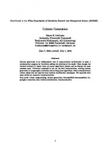
Let us start right away by solving a constrained shortest path problem. Consider the network depicted in Figure 1.1. Besides a cost c ij there is a resource consumption tij attributed to each arc (i, j) ∈ A, say a traversal time. Our goal is to find a shortest path from node 1 to node 6 such that the total traversal time of the path does not exceed 14 time units.

2

4 (1,7)

(2,3)

(1,10)

1

(1,1)

(1,2)

(10,1)

(10,3)

(5,7)

3

(12,3)

5

6

i

(cij , tij )

j

(2,2)

Figure 1.1. Time constrained shortest path problem, Ahuja et al., 1993, p. 599

2 One way to state this particular network flow problem is as the integer program (1.1)–(1.6). One unit of flow has to leave the source (1.2) and has to enter the sink (1.4), while flow conservation (1.3) holds at all other nodes. The time resource constraint appears as (1.5). X

z ? := min

(1.1)

cij xij

(i,j)∈A

subject to

X

x1j = 1

X

xji = 0

X

xi6 = 1

(1.4)

tij xij ≤ 14

(1.5)

(1.2)

j:(1,j)∈A

X

j:(i,j)∈A

xij −

i = 2, 3, 4, 5

(1.3)

j:(j,i)∈A

i:(i,6)∈A

X

(i,j)∈A

xij = 0 or 1

(i, j) ∈ A

(1.6)

An inspection shows that there are nine possible paths, three of which consume too much time. The optimal integer solution is path 13246 of cost 13 with a traversal time of 13. How would we find this out? First note that the resource constraint (1.5) prevents us from solving our problem with a classical shortest path algorithm. In fact, no polynomial time algorithm is likely to exist since the resource constrained shortest path problem is N P-hard. However, since the problem is almost a shortest path problem, we would like to exploit this embedded well-studied structure algorithmically.

1.1

An Equivalent Reformulation: Arcs vs. Paths

If we ignore the complicating constraint (1.5), the easily tractable remainder is X = {xij = 0 or 1 | (1.2)–(1.4)}. It is a well-known result in network flow theory that an extreme point xp = (xpij ) of the polytope defined by the convex hull of X corresponds to a path p ∈ P in the network. This enables us to express any arc flow as a convex combination of path flows: X xij = xpij λp (i, j) ∈ A (1.7) p∈P

X

λp = 1

(1.8)

λp ≥ 0 p ∈ P.

(1.9)

p∈P

3

A Primer in Column Generation

If we substitute for x in (1.1) and (1.5) we obtain the so-called master problem: z ? = min

X X ( cij xpij )λp

(1.10)

X X ( tij xpij )λp ≤ 14

(1.11)

p∈P (i,j)∈A

subject to

p∈P (i,j)∈A

X

(1.12)

λp = 1

p∈P

λp ≥ 0 X

xpij λp = xij

p∈P

(1.13)

(i, j) ∈ A

(1.14)

p∈P

xij = 0 or 1 (i, j) ∈ A .

(1.15)

Loosely speaking, the structural information X that we are looking for a path is hidden in “p ∈ P .” The cost coefficient of λ p is the cost of path p and its coefficient in (1.11) is path p’s duration. Via (1.14) and (1.15) we explicitly preserve the linking of variables (1.7) in the formulation, and we may recover a solution x to our original problem (1.1)–(1.6) from a master problem’s solution. Always remember that integrality must hold for the original x variables.

1.2

The Linear Relaxation of the Master Problem

One starts with solving the linear programming (LP) relaxation of the master problem. If we relax (1.15), there is no longer a need to link the x and λ variables, and we may drop (1.14) as well. There remains a problem with nine path variables and two constraints. Associate with (1.11) and (1.12) dual variables π1 and π0 , respectively. For large networks, the cardinality of P becomes prohibitive, and we cannot even explicitly state all the variables of the master problem. The appealing idea of column generation is to work only with a sufficiently meaningful subset of variables, forming the so-called restricted master problem (RMP). More variables are added only when needed: like in the simplex method we have to find in every iteration a promising variable to enter the basis. In column generation an iteration consists (a) of optimizing the restricted master problem in order to determine the current optimal objective function value z¯ and dual multipliers π, and (b) of finding, if there still is one, a variable λp with negative reduced cost X X c¯p = cij xpij − π1 ( tij xpij ) − π0 < 0. (1.16) (i,j)∈A

(i,j)∈A

The implicit search for a minimum reduced cost variable amounts to optimizing a subproblem, precisely in our case: a shortest path problem in the network of

4 Figure 1.1 with a modified cost structure: X (cij − π1 tij )xij − π0 . c¯? = min (1.2)–(1.4), (1.6)

(1.17)

(i,j)∈A

Clearly, if c¯? ≥ 0 there is no improving variable and we are done with the linear relaxation of the master problem. Otherwise, the variable found is added to the RMP and we repeat. In order to obtain integer solutions to our original problem, we have to embed column generation within a branch-and-bound framework. We now give full numerical details of the solution of our particular instance. We denote by BBn.i iteration number i at node number n (n = 0 represents the root node). The summary in Table 1.1 for the LP relaxation of the master problem also lists the cost cp and duration tp of path p, respectively, and the solution in terms of the value of the original variables x. Table 1.1. BB0: The linear programming relaxation of the master problem Iteration Master Solution z¯ π0 π1 c¯? p cp BB0.1 y0 = 1 100.0 100.00 0.00 −97.0 1246 3 BB0.2 y0 = 0.22, λ1246 = 0.78 24.6 100.00 −5.39 −32.9 1356 24 BB0.3 λ1246 = 0.6, λ1356 = 0.4 11.4 40.80 −2.10 −4.8 13256 15 BB0.4 λ1246 = λ13256 = 0.5 9.0 30.00 −1.50 −2.5 1256 5 BB0.5 λ13256 = 0.2, λ1256 = 0.8 7.0 35.00 −2.00 0 Arc flows: x12 = 0.8, x13 = x32 = 0.2, x25 = x56 = 1

tp 18 8 10 15

Since we have no feasible initial solution at iteration BB0.1, we adopt a bigM approach and introduce an artificial variable y 0 with a large cost, say 100, for the convexity constraint. We do not have any path variables yet and the RMP contains two constraints and the artificial variable. This problem is solved by inspection: y0 = 1, z¯ = 100, and the dual variables are π 0 = 100 and π1 = 0. The subproblem (1.17) returns path 1246 at reduced cost c¯? = −97, cost 3 and duration 18. In iteration BB0.2, the RMP contains two variables: y 0 and λ1246 . An optimal solution with z¯ = 24.6 is y 0 = 0.22 and λ1246 = 0.78, which is still infeasible. The dual variables assume values π 0 = 100 and π1 = −5.39. Solving the subproblem gives the feasible path 1356 of reduced cost −32.9, cost 24, and duration 8. In total, four path variables are generated during the column generation process. In iteration BB0.5, we use 0.2 times the feasible path 13256 and 0.8 times the infeasible path 1256. The optimal objective function value is 7, with π0 = 35 and π1 = −2. The arc flow values provided at the bottom of Table 1.1 are identical to those found when solving the LP relaxation of the original problem.


1.3

5

Branch-and-Bound: The Reformulation Repeats

Except for the integrality requirement (1.6) (or 1.15) all constraints of the original (and of the master) problem are satisfied, and a subsequent branch-andbound process is used to compute an optimal integer solution. Even though it cannot happen for our example problem, in general the generated set of columns may not contain an integer feasible solution. To proceed, we have to start the reformulation and column generation again in each node. Let us first explore some “standard” ways of branching on fractional variables, e.g., branching on x12 = 0.8. For x12 = 0, the impact on the RMP is that we have to remove path variables λ1246 and λ1256 , that is, those paths which contain arc (1, 2). In the subproblem, this arc is removed from the network. When the RMP is re-optimized, the artificial variable assumes a positive value, and we would have to generate new λ variables. On branch x 12 = 1, arcs (1, 3) and (3, 2) cannot be used. Generated paths which contain these arcs are discarded from the RMP, and both arcs are removed from the subproblem. There are also many strategies involving more than a single arc flow variable. One is to branch on the sum of all flow variables which currently is 3.2. Since the solution is a path, an integer number of arcs has to be used, in fact, at least three and at most five in our example. Our freedom of making branching decisions is a powerful tool when properly applied. Alternatively, we branch on x13 + x32 = 0.4. On branch x13 + x32 = 0, we simultaneously treat two flow variables; impacts on the RMP and the subproblem are similar to those described above. On branch x 13 + x32 ≥ 1, this constraint is first added to the original formulation. We exploit again the path substructure X, go through the reformulation process via (1.7), and obtain a new RMP to work with. Details of the search tree are summarized in Table 1.2. At node BB1, we set x13 + x32 = 0. In iteration BB1.1, paths 1356 and 13256 are discarded from the RMP, and arcs (1, 3) and (3, 2) are removed from the subproblem. The resulting RMP with y 0 = 0.067 and λ1256 = 0.933 is infeasible. The objective function assumes a value z¯ = 11.3, and π 0 = 100 and π1 = −6.33. Given these dual multipliers, no column with negative reduced cost can be generated! Here we face a drawback of the big-M approach. Path 12456 is feasible, its duration is 14, but its cost of 14 is larger than the current objective function value, computed as 0.067M + 0.933 × 5. The constant M = 100 is too small, and we have to increase it, say to 1000. (A different phase I approach, that is, minimizing the artificial variable y 0 , would have easily prevented this.) Reoptimizing the RMP in iteration BB1.2 now results in z¯ = 71.3, y 0 = 0.067, λ1256 = 0.933, π0 = 1000, and π1 = −66.33. The subproblem returns path 12456 with a reduced cost of −57.3. In iteration BB1.3, the new RMP has an integer solution λ12456 = 1, with z¯ = 14, an upper bound on the optimal

6 Table 1.2. Details of the branch-and-bound decisions

Iteration Master Solution z¯ π0 π1 π2 c¯? p c p tp BB1: BB0 and x13 + x32 = 0 BB1.1 y0 = 0.067, λ1256 = 0.933 11.3 100 −6.33 – 0 BB1.2 Big-M increased to 1000 y0 = 0.067, λ1256 = 0.933 71.3 1000 −66.33 – −57.3 12456 14 14 BB1.3 λ12456 = 1 14 1000 −70.43 – 0 BB2: BB0 and x13 + x32 ≥ 1 BB2.1 λ1246 = λ13256 = 0.5 9 15 −0.67 3.33 0 Arc flows: x12 = x13 = x24 = x25 = x32 = x46 = x56 = 0.5 BB3: BB2 and x12 = 0 BB3.1 λ13256 = 1 15 15 0 0 -2 13246 13 13 BB3.2 λ13246 = 1 13 13 0 0 0 BB4: BB2 and x12 = 1 BB4.1 y0 = 0.067, λ1256 = 0.933 111.3 100 −6.33 100 0 Infeasible arc flows

path cost. The dual multipliers are π 0 = 1000 and π1 = −70.43, and no new variable is generated. At node BB2, we impose x13 +x32 ≥ 1 to the original formulation, and again, we reformulate these x variables in terms of the λ variables. The resulting new P constraint (with dual multiplier π 2 ) in the RMP is p∈P (xp13 + xp32 )λp ≥ 1. From the value of (xp13 + xp32 ) we learn how often arcs (1, 3) and (3, 2) are used in path p. The current problem at node BB2.1 is the following: min 100y0 subject to:

+

3λ1246 18λ1246

y0 + y0 ,

+ 24λ1356 + 8λ1356 λ1356 λ1246 + λ1356 λ1246 , λ1356 ,

+ 15λ13256 + 5λ1256 + 10λ13256 + 15λ1256 + 2λ13256 + λ13256 + λ1256 λ13256 , λ1256

≤ 14 ≥ 1 = 1 ≥ 0

[π1 ] [π2 ] [π0 ]

From solving this linear program we obtain an increase in the objective function z¯ from 7 to 9 with variables λ 1246 = λ13256 = 0.5, and dual multipliers π0 = 15, π1 = −0.67, and π2 = 3.33. The new subproblem is given by X c¯? = min (cij − π1 tij )xij − π0 − π2 (x13 + x32 ). (1.18) (1.2)–(1.4), (1.6)

(i,j)∈A

For these multipliers no path of negative reduced cost exists. The solution of the flow variables is x12 = x13 = x24 = x25 = x32 = x46 = x56 = 0.5. Next, we arbitrarily choose variable x 12 = 0.5 to branch on. Two iterations are needed when x12 is set to zero. In iteration BB3.1, path variables λ 1246

7


and λ1256 are discarded from the RMP and arc (1, 2) is removed from the subproblem. The RMP is integer feasible with λ 13256 = 1 at cost 15. Dual multipliers are π0 = 15, π1 = 0, and π2 = 0. Path 13246 of reduced cost −2, cost 13 and duration 13 is generated and used in the next iteration BB3.2. Again the RMP is integer feasible with path variable λ 13246 = 1 and a new best integer solution at cost 13, with dual multipliers π 0 = 15, π1 = 0, and π2 = 0 for which no path of negative reduced cost exists. On the alternative branch x12 = 1 the RMP is optimal after a single iteration. In iteration BB4.1, variable x13 can be set to zero and variables λ1356 , λ13256 , and λ13246 are discarded from the current RMP. After the introduction of an artificial variable y2 in the second row, the RMP is infeasible since y 0 > 0 (as can be seen also from the large objective function value z¯ = 111.3). Given the dual multipliers, no columns of negative reduced cost can be generated, and the RMP remains infeasible. The optimal solution (found at node BB3) is path 13246 of cost 13 with a duration of 13 as well.

2.

Some Theoretical Background

In the previous example we already saw all the necessary building blocks for a column generation based solution approach to integer programs: (1) an original formulation to solve which acts as the control center to facilitate the design of natural branching rules and cutting planes; (2) a master problem to determine the currently optimal dual multipliers and to provide a lower bound at each node of the branch-and-bound tree; (3) a pricing subproblem which explicitly reflects an embedded structure we wish to exploit. In this section we detail the underlying theory.

2.1

Column Generation

Let us call the following linear program the master problem (MP). X ? zM cj λj P := min subject to

j∈J X

aj λj

≥ b

(1.19)

j∈J

λj

≥ 0, j ∈ J.

In each iteration of the simplex method we look for a non-basic variable to price out and enter the basis. That is, given the non-negative vector π of dual variables we wish to find a j ∈ J which minimizes c¯j := cj − π t aj . This explicit pricing is a too costly operation when |J| is huge. Instead, we work with a reasonably small subset J 0 ⊆ J of columns—the restricted master problem (RMP)—and evaluate reduced costs only by implicit enumeration. Let λ and π assume primal and dual optimal solutions of the current RMP, respectively. When

8 columns aj , j ∈ J, are given as elements of a set A, and the cost coefficient c j can be computed from aj via a function c then the subproblem c¯? := min c(a) − π t a | a ∈ A (1.20)

performs the pricing. If c¯? ≥ 0, there is no negative c¯j , j ∈ J, and the solution λ to the restricted master problem optimally solves the master problem as well. Otherwise, we add to the RMP the column derived from the optimal subproblem solution, and repeat with re-optimizing the RMP. The process is initialized with an artificial, a heuristic, or a previous (“warm start”) solution. In what regards convergence, note that each a ∈ A is generated at most once since no variable in an optimal RMP has negative reduced cost. When dealing with some finite set A (as is practically always true), the column generation algorithm is exact. In addition, we can make use of bounds. Let z¯ denoteP the optimal objective function value to the RMP. When an upper bound κ ≥ j∈J λj holds for the optimal solution of the master problem, we have not only an upper bound z¯ on ? zM ¯ by more P in each iteration, but also a lower bound: we cannot reduce z than κ times the smallest reduced cost c¯? : ? z¯ + κ¯ c ? ≤ zM ¯. P ≤z

(1.21)

Thus, we may verify the solution quality at any time. In the optimum of (1.19), ? . c¯? = 0 for the basic variables, and z¯ = z M P

2.2

Dantzig-Wolfe Decomposition for Integer Programs

In many applications we are interested in optimizing over a discrete set X. For X = {x ∈ Zn+ | Dx ≥ d} 6= ∅ we have the special case of integer linear programming. Consider the following (original or compact) program: z ? := min ct x subject to Ax ≥ b x ∈ X.

(1.22)

Replacing X by conv(X) in (1.22) does not change z ? which we assume to be finite. The Minkowski and Weyl theorems (see Schrijver, 1986) enable us to represent each x ∈ X as a convex combination of extreme points {x p }p∈P plus a non-negative combination of extreme rays {x r }r∈R of conv(X), i.e., X X X |P |+|R| x= xp λp + xr λr , λp = 1, λ ∈ R+ (1.23) p∈P

r∈R

p∈P

where the index sets P and R are finite. Substituting for x in (1.22) and applying the linear transformations cj = ct xj and aj = Axj , j ∈ P ∪ R we obtain an

9


equivalent extensive formulation X X z ? := min cp λp + cr λr p∈P

subject to

X

(1.24)

r∈R

ap λp +

p∈P

X

ar λr ≥ b

(1.25)

=1

(1.26)

λ ≥0

(1.27)

xr λr = x

(1.28)

r∈R

X

λp

p∈P

X

p∈P

xp λp +

X

r∈R

x ∈ Zn+ .

(1.29)

Equation (1.26) is referred to as the convexity constraint. When we relax the integrality of x, there is no need to link x and λ, and we may also relax (1.28). The columns of this special master problem are defined by the extreme points and extreme rays of conv(X). We solve the master by column generation to ? . Given an optimal dual solution get its optimal objective function value z M P π and π0 to the current RMP, where variable π 0 corresponds to the convexity constraint, the subproblem is to determine min j∈P {cj − π t aj − π0 } and minj∈R {cj − π t aj }. By our previous linear transformation and since π 0 is a constant, this results in c¯? := min (ct − π t A)x − π0 | x ∈ X . (1.30)

This subproblem is an integer linear program. When c¯? ≥ 0, there is no negative reduced cost column, and the algorithm terminates. When c¯? < 0 and finite, an optimal solution to (1.30) is an extreme point x p of conv(X), and we add the column [ct xp , (Axp )t , 1]t to the RMP. When c¯? = −∞ we identify an extreme ray xr of conv(X) as a solution x ∈ X to (ct − π t A)x = 0, and add the column [ct xr , (Axr )t , 0]t to the RMP. From (1.21) together with the convexity constraint we obtain in each iteration ? ¯, z¯ + c¯? ≤ zM P ≤z

(1.31)

where z¯ = π t b + π0 is again the optimal objective function value of the RMP. ? ? ¯+ c Since zM ¯? is also a lower bound on z ? . In general, z¯ is not a valid P ≤ z ,z ? upper bound on z , except if the current x variables are integer. The algorithm is exact and finite as long as finiteness is ensured in optimizing the RMP. The original formulation is the starting point to obtain integer solutions in the x variables. Branching and cutting constraints are added there, the reformulation as in Section 1.1.1 is re-applied, and the process continues with an updated

10 master problem. It is important to see that it is our choice as to whether the additional constraints remain in the master problem (as in the previous section) or go into the subproblem (as we will see later).

Pricing Out the Original x Variables. Assume that in (1.22) we have a linear subproblem X = {x ∈ Rn+ | Dx ≥ d} 6= ∅. Column generation then essentially solves the linear program min ct x subject to

Ax ≥ b, Dx ≥ d, x ≥ 0.

We obtain an optimal primal solution x but only the dual multipliers π associated with the constraint set Ax ≥ b. However, following an idea of Walker, 1969 we can also retrieve the dual variables σ associated with Dx ≥ d: it is the vector obtained from solving the linear subproblem in the last iteration of the column generation process. This full dual information allows for a pricing of the original variables, and therefore a possible elimination of some of them. Given an upper bound on the integer optimal objective function value of the original problem, one can eliminate an x variable if its reduced cost is larger than the optimality gap. In the general case of a linear integer or even non-linear pricing subproblem, the above procedure does not work. Poggi de Aragão and Uchoa, 2003 suggest to directly use the extensive formulation: if we keep the coupling constraint (1.28) in the master problem, it suffices to impose the constraint x ≥ , for a small > 0, at the end of the process. The shadow prices of these constraints are the reduced costs of the x vector of original variables. Note that there is no need to apply the additional constraints to already positive variables. Computational experiments underline the benefits of this procedure.

Block Diagonal Structure. For practical problems Dantzig-Wolfe decomposition can typically exploit a block diagonal structure of D, i.e.,  1    1 d D 2  2    D  d    (1.32) d = D=    . ..   ..   . Dκ

dκ .

Each X k = {D k xk ≥ dk , xk ≥ 0 and integer}, k ∈ K := {1, . . . , κ}, gives rise to a representation as in (1.23). The decomposition yields κ subproblems, each with its own convexity constraint and associated dual variable: c¯k? := min{(ckT − π t Ak )xk − π0k | xk ∈ X k }, k ∈ K.

(1.33)

The superscript k to all entities should be interpreted in the canonical way. The algorithm terminates when c¯k? ≥ 0, for all k ∈ K. Otherwise, extreme points

11


and rays identified in (1.33) give rise to new P columns to be added to the RMP. By linear programming duality, z¯ = π t b + κk=1 π0k , and we obtain the following bounds, see Lasdon, 1970: z¯ +

κ X

? c¯k? ≤ zM ¯. P ≤z

(1.34)

k=1

2.3

Useful Working Knowledge

When problems get larger and computationally much more difficult than our small constrained shortest path problem it is helpful to know more about mechanisms, their consequences, and how to exploit them.

Infeasible paths. One may wonder why we kept infeasible paths in the RMP during column generation. Here, as for the whole process, we cannot overemphasize the fact that knowledge about the integer solution usually does not help us much in solving the linear relaxation program. Figure 1.2 illustrates the domain of the RMP (shaded) and the domain X of the subproblem. In part (a), the optimal solution x, symbolized by the dot, is uniquely determined as a convex combination of the three extreme points of the triangle X, even though all of them are not feasible for the intersection of the master and subproblem. In our example, in iteration BB0.5, any convex combination of feasible paths which have been generated, namely 13256 and 1356, has cost larger than 7, i.e., is suboptimal for the linear relaxation of the master problem. Infeasible paths are removed only if needed during the search for an integer solution. In Figure 1.2 (a), x can be integer and no branch-and-bound search is needed. In part (b) there are many ways to express the optimal solution as a convex combination of three extreme points. This is a partial explanation of the slow convergence (tailing off ) of linear programming column generation.

X

X

x

master

x

master (a)

(b)

Figure 1.2. Schematic illustration of the domains of master and subproblem X

12 Lower and Upper Bounds. Figure 1.3 gives the development of upper (¯ z) ? and lower (¯ z + c¯∗ ) bounds on zM in the root node for our small constrained P shortest path example. The values for the lower bound are 3.0, −8.33, 6.6, 6.5, and finally 7. While the upper bound decreases monotonically (as expected when minimizing a linear program) there is no monotony for the lower bound. Still, we can use these bounds to evaluate the quality of the current solution by computing the optimality gap, and could stop the process when a preset quality is reached. Is there any use of the bounds beyond that? Note first that U B = z¯ 100

z¯ z¯ + c¯?

80 60 40 20 0 -20

1

2

3 Iterations

4

5

Figure 1.3. Development of lower and upper bounds on zM P in BB0

is not an upper bound on z ? . The currently (over all iterations) best lower bound ? ? LB, however, is a lower bound on zM P and on z . Even though there is no direct use of LB or U B in the master problem we can impose the additional constraints LB ≤ ct x ≤ U B to the subproblem structure X if the subproblem consists of a single block. Be aware that this cutting modifies the subproblem structure X, with all algorithmic consequences, that is, possible complications for a combinatorial algorithm. In our constrained shortest path example, two generated paths are feasible and provide upper bounds on the optimal integer solution z ∗ . The best one is path 13256 of cost 15 and duration 10. Table 1.3 shows the multipliers σi , i = 1, . . . , 6 for the flow conservation constraints of the path structure X at the last iteration of the column generation process.

Table 1.3. Multipliers σi for the flow conservation constraints on nodes i ∈ N node i 1 2 3 4 5 6 σi 29 8 13 5 0 −6


13

Therefore, given the optimal multiplier π 1 = −2 for the resource constraint, the reduced cost of an arc is given by c¯ij = cij − σi + σj − tij π1 , (i, j) ∈ A. The reader can verify that c¯34 = 3 − 13 + 5 − (7)(−2) = 11. This is the only reduced cost which exceeds the current optimality gap which equals to 15 − 7 = 8. Arc (3, 4) can be permanently discarded from the network and paths 1346 and 13456 will never be generated.

Integrality Property. Solving the subproblem as an integer program usually helps in closing part of the integrality gap of the master problem (Geoffrion, 1974), except when the subproblem possesses the integrality property. This property means that solutions to the pricing problem are naturally integer when it is solved as a linear program. This is the case for our shortest path subproblem and this is why we obtained the value of the linear relaxation of the original problem as the value of the linear relaxation of the master problem. When looking for an integer solution to the original problem, we need to impose new restrictions on (1.1)–(1.6). One way is to take advantage of a new X structure. However, if the new subproblem is still solved as a linear program, ? zM P remains 7. Only solving the new X structure as an integer program may ? improve zM P . Once we understand that we can modify the subproblem structure, we can devise other decomposition strategies. One is to define the X structure as X tij xij ≤ 14, xij binary, (i, j) ∈ A (1.35) (i,j)∈A

so that the subproblem becomes a knapsack problem which does not possess the ? integrality property. Unfortunately, in this example, z M P remains 7. However, improvements can be obtained by imposing more and more constraints to the subproblem. An example is to additionally enforce the selection of one arc to leave the source P (1.2) and another one to enter the sink (1.4), and impose constraint 3 ≤ (i,j)∈A xij ≤ 5 on the minimum and maximum number of selected arcs. Richer subproblems, as long as they can be solved efficiently and do not possess the integrality property, may help in closing the integrality gap. It is also our decision how much branching and cutting information (ranging from none to all) we put into the subproblem. This choice depends on where the additional constraints are more easily accommodated in terms of algorithms and computational tractability. Branching decisions imposed on the subproblem can reduce its solution space and may turn out to facilitate a solution as integer program. As an illustration we describe adding the lower bound cut in the root node of our small example.

Imposing the Lower Bound Cut ct x ≥ 7. Assume that we have solved the relaxed RMP in the root node and instead of branching, we impose the lower

14 bound cut on the X structure, see Table 1.4. Note that this cut would not have helped in the RMP since z¯ = ct x = 7 already holds. We start modifying the RMP by removing variables λ1246 and λ1256 as their cost is smaller than 7. In iteration BB0.6, for the re-optimized RMP λ 13256 = 1 is optimal at cost 15; it corresponds to a feasible path of duration 10. U B is updated to 15 and the dual multipliers are π0 = 15 and π1 = 0. The X structure is modified by adding constraint ct x ≥ 7. Path 13246 is generated with reduced cost −2, cost 13, and duration 13. The new lower bound is 15 − 2 = 13. On the downside of this significant improvement is the fact that we have destroyed the pure network structure of the subproblem which we have to solve as an integer program now. We may pass along with this circumstance if it pays back a better bound. We re-optimize the RMP in iteration BB0.7 with the added variable λ 13246 . This variable is optimal at value 1 with cost and duration equal to 13. Since this variable corresponds to a feasible path, it induces a better upper bound which is equal to the lower bound: optimality is proven. There is no need to solve the subproblem. Table 1.4. Lower bound cut added to the subproblem at the end of the root node Iteration Master Solution z¯ π0 π1 c¯? p cp tp U B LB BB0.6 λ13256 = 1 15 15 0 −2 13246 13 13 15 13 BB0.7 λ13246 = 1 13 13 0 13 13

Note that using the dynamically adapted lower bound cut right from the start has an impact on the solution process. For example, the first generated path 1246 would be eliminated in iteration BB0.3 since the lower bound reaches 6.6, and path 1256 is never generated. Additionally adding the upper bound cut has a similar effect.

Acceleration Strategies. Often acceleration techniques are key elements for the viability of the column generation approach. Without them, it would have been almost impossible to obtain quality solutions to various applications, in a reasonable amount of computation time. We sketch here only some strategies, see e.g., Desaulniers et al., 2001 for much more. The most widely used strategy is to return to the RMP many negative reduced cost columns in each iteration. This generally decreases the number of column generation iterations, and is particularly easy when the subproblem is solved by dynamic programming. When the number of variables in the RMP becomes too large, non-basic columns with current reduced cost exceeding a given threshold may be removed. Accelerating the pricing algorithm itself usually yields most significant speed-ups. Instead of investing in a most negative reduced cost

15


column, any variable with negative reduced cost suffices. Often, such a column can be obtained heuristically or from a pool of columns containing not yet used columns from previous calls to the subproblem. In the case of many subproblems, it is often beneficial to consider only few of them each time the pricing problem is called. This is the well-known partial pricing. Finally, in order to reduce the tailing off behavior of column generation, a heuristic rule can be devised to prematurely stop the linear relaxation solution process, for example, when the value of the objective function does not improve sufficiently in a given number of iterations. In this case, the approximate LP solution does not necessarily provide a lower bound but using the current dual multipliers, a lower bound can still be computed. With a careful use of these ideas one may confine oneself with a non-optimal solution in favor of being able to solve much larger problems. This turns column generation into optimization based heuristics which may be used for comparison with other methods for a given class of problems.

3.

A Dual Point of View

The dual program of the RMP is a relaxation of the dual of the master problem, since constraints are omitted. Viewing column generation as row generation in the dual, it is a special case of Kelley’s cutting plane method from 1961. Recently, this dual perspective attracted considerable attention and we will see that it provides us with several key insights. Observe that the generation process as well as the stopping criteria are driven entirely by the dual multipliers.

3.1

Lagrangian Relaxation

A practically often used dual approach to solving (1.22) is Lagrangian relaxation, see Geoffrion, 1974. Penalizing the violation of Ax ≥ b via Lagrangian multipliers π ≥ 0 in the objective function results in the Lagrangian subproblem relative to constraint set Ax ≥ b L(π) := min ct x − π t (Ax − b). x∈X

(1.36)

Since L(π) ≤ min{ct x − π t (Ax − b) | Ax ≥ b, x ∈ X} ≤ z ? , L(π) is a lower bound on z ? . The best such bound on z ? is provided by solving the Lagrangian dual problem L := max L(π). (1.37) π ≥0 Note that (1.37) is a problem in the dual space while (1.36) is a problem in x. The Lagrangian function L(π), π ≥ 0 is the lower envelope of a family of functions linear in π, and therefore is a concave function of π. It is piecewise linear with breakpoints where the optimal solution of L(π) is not unique. In particular, L(π) is not differentiable, but only sub-differentiable. The most popular, since

16 very easy to implement, choice to obtain optimal or near optimal multipliers are subgradient algorithms. However, let us describe an alternative computation method, see Nemhauser and Wolsey, 1988. We know that replacing X by conv(X) in (1.22) does not change z ? and this will enable us to write (1.37) as a linear program. When X = ∅, which may happen during branch-and-bound, then L = ∞. Otherwise, given some multipliers π, the Lagrangian bound is −∞ if (ct − π t A)xr < 0 for some r ∈ R L(π) = t t c xp − π (Axp − b) for some p ∈ P otherwise. Since we assumed z ? to be finite, we avoid unboundedness by writing (1.37) as max min ct xp − π t (Axp − b) such that (ct − π t A)xr ≥ 0, ∀r ∈ R, π ≥0 p∈P or as a linear program with many constraints L = max π0 subject to π t (Axp − b) + π0 ≤ ct xp , p ∈ P π t Axr ≤ c t xr , r ∈ R π ≥ 0.

(1.38)

The dual of (1.38) reads as the linear relaxation of the master problem (1.24)– (1.29): X X L = min ct xp λp + ct xr λr subject to

p∈P X

Axp λp +

p∈P

r∈R X

Axr λr ≥ b

r∈R

X

λp

p∈P

X

p∈P

(1.39)

λp = 1 λ ≥ 0.

Observe that for a given vector π of multipliers and a constant π 0 , L(π) = (π t b + π0 ) +

min

x∈conv(X)

(ct − π t A)x − π0 = z¯ + c¯? ,

that is, each time the RMP is solved during the Dantzig-Wolfe decomposition, the computed lower bound in (1.31) is the same as the Lagrangian bound, that is, for optimal x and π we have z ? = ct x = L(π). When we apply Dantzig-Wolfe decomposition to (1.22) we satisfy complementary slackness conditions, we have x ∈ conv(X), and we satisfy Ax ≥ b. Therefore only the integrality of x remains to be checked. The situation is different for subgradient algorithms. Given optimal multipliers π for (1.37),


17

we can solve (1.36) which ensures that the solution, denoted x π , is (integer) feasible for X and π t (Axπ − b) = 0. Still, we have to check whether the relaxed constraints are satisfied, that is, Ax π ≥ b to prove optimality. If this condition is violated, we have to recover optimality of a primal-dual pair (x, π) by branch-and-bound. For many applications, one is able to slightly modify infeasible solutions obtained from the Lagrangian subproblems with only a small degradation of the objective value. Of course these are only approximate solutions to the original problem. We only remark that there are more advanced (non-linear) alternatives to solve the Lagrangian dual like the bundle method (Hiriart-Urruty and Lemaréchal, 1993) based on quadratic programming, and the analytic center cutting plane method (Goffin and Vial, 1999), an interior point solution approach. However, the performance of these methods is still to be evaluated in the context of integer programming.

3.2

Dual Restriction / Primal Relaxation

Linear programming column generation remained “as is” for a long time. Recently, the dual point of view prepared the ground for technical advances.

Structural Dual Information. Consider a master problem and its dual and assume both are feasible and bounded. In some situations we may have additional knowledge about an optimal dual solution which we may express as additional valid inequalities F t π ≤ f in the dual. To be more precise, we would like to add inequalities which are satisfied by at least one optimal dual solution. Such valid inequalities correspond to additional primal variables y ≥ 0 of cost f that are not present in the original master problem. From the primal perspective, we therefore obtain a relaxation. Devising such dual-optimal inequalities requires (but also exploits) a specific problem knowledge. This has been successfully applied to the one-dimensional cutting stock problem, see Valério de Carvalho, 2003 and Ben Amor et al., 2003. Oscillation. It is an important observation that the dual variable values do not develop smoothly but they very much oscillate during column generation. In the first iterations, the RMP contains too few columns to provide any useful dual information, in turn resulting in non useful variables to be added. Initially, often the penalty cost of artificial variables guide the values of dual multipliers (Vanderbeck, 2005 calls this the heading-in effect). One observes that the variables of an optimal master problem solution are generated in the last iterations of the process when dual variables finally come close to their respective optimal values. Understandably, dual oscillation has been identified as a major efficiency issue. One way to control this behavior is to impose lower and upper bounds, that is, we constrain the vector of dual variables to lie “in a box” around its current value. As a result, the RMP is modified by adding slack

18 and surplus variables in the corresponding constraints. After re-optimization of the new RMP, if the new dual optimum is attained on the boundary of the box, we have a direction towards which the box should be relocated. Otherwise, the optimum is attained in the box’s interior, producing the global optimum. This is the principle of the Boxstep method (Marsten, 1975; Marsten et al., 1975).

Stabilization. Stabilized column generation (see du Merle et al., 1999; Ben Amor and Desrosiers, 2003) offers more flexibility for controlling the duals. Again, the dual solution π is restricted to stay in a box, however, the box may be left at a certain penalty cost. This penalty may be a piecewise linear function. The size of the box and the penalty are updated dynamically so as to make greatest use of the latest available information. With intent to reduce the dual variables’ variation, select a small box containing the (in the beginning estimated) current dual solution, and solve the modified master problem. Componentwise, if the new dual solution lies in the box, reduce its width and increase the penalty. Otherwise, enlarge the box and decrease the penalty. This allows for fresh dual solutions when the estimate was bad. The update could be performed in each iteration, or alternatively, each time a dual solution of currently best quality is obtained.

3.3

Dual Aspects of our Shortest Path Example

Optimal Primal Solutions. Assume that we penalize the violation of resource constraint (1.5) via the objective function with the single multiplier π1 ≤ 0 which we determine using a subgradient method. Its optimal value is π1 = −2, as we know from solving the primal master problem by column generation. The aim now is to find an optimal integer solution x to our original problem. From the Lagrangian subproblem with π 1 we get L(−2) = 7 and generate either the infeasible path 1256 of cost 5 and duration 15, or the feasible path 13256 of cost 15 and duration 10. The important issue now, left out in textbooks, is how to perform branch-and-bound in that context? Assume that we generated path 1256. A possible strategy to start the branchand-bound search tree is to introduce cut x 12 + x25 + x56 ≤ 2 in the original formulation (1.1)–(1.6), and then either incorporate it in X or relax it (and penalize its violation) in the objective function via a second multiplier. The first alternative prevents the generation of path 1256 for any value of π 1 . However, we need to re-compute its optimal value according to the modified X structure, i.e., π1? = −1.5. In this small example, a simple way to get this value is to solve the linear relaxation of the full master problem excluding the discarded path. Solving the new subproblem results in an improved lower bound L(−1.5) = 9, and the generated path 13256 of cost 15 and duration 10. This path is feasible but suboptimal. In fact, this solution x is integer, satisfies the path constraints but does not satisfy complementary slackness for the resource constraint. That


19

P is, π1 ( (i,j)∈A tij xij − 14) = −1.5(10 − 14) 6= 0. The second cut x 13 + x32 + x25 + x56 ≤ 3 in the X structure results in π1? = −2, an improved lower bound of L(−2) = 11, and the generated path 1246 of cost 3 and duration 18. This path is infeasible, and adding the third cut x 12 + x24 + x46 ≤ 2 in the subproblem X gives us the optimal solution, that is, π 1 = 0, L(0) = 13 with the generated path 13245 of cost 13 and duration 13. Alternatively, we could have penalized the cuts via the objective function which would not have destroyed the subproblem structure. We encourage the reader to find the optimal solution this way, making use of any kind of branching and cutting decisions that can be defined on the x variables.

A Box Method. It is worthwhile to point out that a good deal of the operations research literature is about Lagrangian relaxation. We can steal ideas there about how to decompose problems and use them in column generation algorithms (see Guignard, 2004). In fact, the complementary availability of both, primal and dual ideas, brings us in a strong position which e.g., motivates the following. Given optimal multipliers π obtained by a subgradient algorithm, one can use very small boxes around these in order to rapidly derive an optimal primal solution x on which branching and cutting decisions are applied. The dual information is incorporated in the primal RMP in the form of initial columns together with the columns corresponding to the generated subgradients. This gives us the opportunity to initiate column generation with a solution which intuitively bears both, relevant primal and dual information. Alternatively, we have applied a box method to solve the primal master problem by column generation, c.f. Table 1.5. We impose the box constraint −2.1 ≤ π1 ≤ −1.9. At start, the RMP contains the artificial variable y 0 in the convexity constraint, and surplus (s 1 with cost coefficient 1.9) and slack (s 2 with cost coefficient 2.1) variables in the resource constraint. Table 1.5. A box method in the root node with −2.1 ≤ π1 ≤ −1.9

Iteration Master Solution z¯ π0 π1 c¯? p c p tp U B BoxBB0.1 y0 = 1, s2 = 14 73.4 100.0 −1.9 −66.5 1256 5 15 – BoxBB0.2 λ1256 = 1, s1 = 1 7.1 36.5 −2.1 −0.5 13256 15 10 7.1 BoxBB0.3 λ13256 = 0.2, λ1256 = 0.8 7.0 35.0 −2.0 0 7 Arc flows: x12 = 0.8, x13 = x32 = 0.2, x25 = x56 = 1

LB 6.9 6.6 7

In the first iteration, denoted BoxBB0.1, the artificial variable y 0 = 1 and the slack variable s2 = 14 constitute a solution. The current dual multipliers are π0 = 100 and π1 = −1.9. Path 1256 is generated (cost 5 and duration 15) and the lower bound already reaches 6.9. In the second iteration, λ 1256 = 1 and

20 surplus s1 = 1 define an optimal solution to the RMP. This solution provides an upper bound of 7.1 and dual multipliers are π 0 = 36.5 and π1 = −2.1. Experimentation reveals that a smaller box around π = −2 results in a smaller optimality gap. The subproblem generates path 13256 (cost 15 and duration 10) and the lower bound decreases to 6.6. Solving the RMP in BoxBB0.3 gives us an optimal solution of the linear relaxation of the master problem. This can be verified in two ways: the previous lower bound values 6.9 and 6.6, rounded up, equal the actual upper bound z¯ = 7; and the reduced cost of the subproblem is zero. Hence, the solution process is completed in only three iterations! The box constraint has to be relaxed when branch-and-bound starts but this does not require any re-optimization iteration.

Geometric Interpretation. Let us draw the Lagrangian function L(π), for π ≤ 0, for our numerical example, where π ≡ π 1 . Since the polytope X is bounded, there are no extreme rays and L(π) can be written in terms of the nine possible extreme points (paths). That is, L(π) = min p∈P cp + (14 − tp )π, where cp and tp are the cost and duration of path p, respectively. Table 1.6 lists the lines (in general, hyperplanes) defined by p ∈ P , with an intercept of c p and a slope of 14 − tp . We have plotted these lines in Figure 1.4. Table 1.6. Hyperplanes (lines) defined by the extreme points of X, i.e., by the indicated paths p 1246 1256 12456 13246 13256 132456 1346 13456 1356 line 3 − 4π 5 − π 14 13 + π 15 + 4π 24 + 5π 16 − 3π 27 + π 24 + 6π

Observe that for π given, the line of smallest cost defines the value of function L(π). The Lagrangian function L(π) is therefore the lower envelope of all lines and its topmost point corresponds to the value L of the Lagrangian dual problem. If one starts at π = 0, the largest possible value is L(0) = 3, on the line defined by path 1246. At that point the slope is negative (the line is defined by 3−4π) so that the next multiplier should be found on the left to the current point. In Dantzig-Wolfe decomposition, we found π(≡ π 1 ) = −97/18 ≈ −5.4. This result depends on big M : the exact value of the multiplier is (3 − M )/18. For any large M , path 1356 is returned, and here, L(−97/18) = −25/3, a lesser lower bound on L(π). The next multiplier is located where the two previous lines intersect, that is, where 3 − 4π = 24 + 6π for π = −2.1. L(−2.1) = 6.6 for path 13256 with an improvement on the lower bound. In the next iteration, the optimal multiplier value is at the intersection of the lines defined by paths 1246 and 13256, that is, 3 − 4π = 15 + 4π for π = −1.5. For that value, the Lagrangian function reaches 6.5 for path 1256. The final and optimal Lagrangian multiplier is at the

21

A Primer in Column Generation Paths 1-3-4-6

30

1-2-4-6 1-3-4-5-6 1-2-4-5-6 1-2-5-6

10

1-3-2-4-6 1-3-2-4-5-6

0

Lagrangian function L(π)

cp + (14 − tp )π

20

1-3-2-5-6 1-3-5-6

−6

−10 −5

−4

−3

−2

−1

0

Lagrangian multiplier π Figure 1.4. Lagrangian function L(π)

intersection of the lines defined by paths 13256 and 1256, that is, 15+4π = 5−π for π = −2 and therefore L(−2) = 7. We can now see why the lower bound is not strictly increasing: the point associated with the Lagrangian multiplier moves from left to right, and the value of the Lagrangian function is determined by the lowest line which is hit. The Lagrangian point of view also teaches us why two of our methods are so successful: when we used the box method for solving the linear relaxation of the master problem by requiring that π has to lie in the small interval [−2.1, −1.9] around the optimal value π = −2, only two paths are sufficient to describe the lower envelope of the Lagrangian function L(π). This explains the very fast convergence of this stabilization approach. Also, we previously added the cut ct x ≥ 7 in the subproblem, when we were looking for an integer solution to our resource constrained shortest path problem. In Figure 1.4 this corresponds to removing the two lines with an intercept smaller than 7, that is, for paths 1246 and 1256. The maximum value of function L(π) is now attained for π = 0 and L(0) = 13.

22

4.

On Finding a Good Formulation

Many vehicle routing and crew scheduling problems, but also many others, possess a multicommodity flow problem as an underlying basic structure (see Desaulniers et al., 1998). Interestingly, Ford and Fulkerson, 1958, suggested to solve this “problem of some importance in applications” via a “specialized computing scheme that takes advantage of the structure”: the birth of column generation which then inspired Dantzig and Wolfe, 1960 to generalize the framework to a decomposition scheme for linear programs as presented in Section 1.2.1. Ford and Fulkerson had no idea “whether the method is practicable.” In fact, at that time, it was not. Not only because of the lack of powerful computers but mainly because (only) linear programming was used to attack integer programs: “That integers should result as the solution of the example is, of course, fortuitous” (Gilmore and Gomory, 1961). In this section we stress the importance (and the efforts) to find a “good” formulation which is amenable to column generation. Our example is the classical column generation application, see Ben Amor and Valério de Carvalho, 2005. Given a set of rolls of width L and integer demands n i for items of length ì , i ∈ I the aim of the cutting stock problem is to find patterns to cut the rolls to fulfill the demand while minimizing the number of used rolls. An item may appear more than once in a cutting pattern and a cutting pattern may be used more than once in a feasible solution.

4.1

Gilmore and Gomory (1961, 1963)

Let R be the set of all feasible cutting patterns. Let coefficient a ir denote how often item i ∈ I is used P in pattern r ∈ R. Feasibility of r is expressed by the knapsack constraint i∈I air ì ≤ L. The classical formulation of Gilmore and Gomory (1961, 1963) makes use of non-negative integer variables: λ r reflects how often pattern r is cut in the solution. We are first interested in solving the linear relaxation of that formulation by column generation. Consider the following primal and dual linear master problems P CS and DCS , respectively: P P (PCS ) : min r∈R λr i∈I r∈R air λr ≥ ni , λr ≥ 0, r∈R

P (DCS ) : max i∈I ni πi P i∈I air πi ≤ 1, r ∈ R πi ≥ 0, i ∈ I .

For i ∈ I, let πi denote the associated dual multiplier, and let x i count the frequency item i is selected in a pattern. Negative reduced cost patterns are generated by solving X X X min 1 − πi xi ≡ max πi xi such that xi ì ≤ L, xi ∈ Z+ , i ∈ I. i∈I

i∈I

i∈I

23


This pricing subproblem is a knapsack problem and the coefficients of the generated columns are given by the value of variables x i , i ∈ I. Gilmore and Gomory, 1961 showed that equality in the demand constraints can be replaced by greater than or equal. Column generation is accelerated by this transformation: dual variables π i , i ∈ I then assume only non-negative values and it is easily shown by contradiction that these dual non-negativity constraints are satisfied by all optimal solutions. Therefore they define a set of (simple) dual-optimal inequalities. Although PCS is known to provide a strong lower bound on the optimal number of rolls, its solution can be fractional and one has to resort to branchand-bound. In the literature one finds several tailored branching strategies based on decisions made on the λ variables, see Barnhart et al., 1998; Vanderbeck and Wolsey, 1996. However, we have seen that branching rules with a potential for exploiting more structural information can be devised when some compact formulation is available.

4.2

Kantorovich (1939, 1960)

From a technical point of view, the proposal by Gilmore and Gomory is a master problem and a pricing subproblem. For precisely this situation, Villeneuve et al., 2003 show that an equivalent compact formulation exists under the assumption that the sum of the variables of the master problem be bounded by an integer κ and that we have the possibility to also bound the domain of the subproblem. The variables and the domain of the subproblem are duplicated κ times, and the resulting formulation has a block diagonal structure with κ identical subproblems. Formally, when we start from Gilmore and Gomory’s formulation, this yields the following formulation of the cutting stock problem. Given the dual multipliers πi , i ∈ I, the pricing subproblem can alternatively be written as X min (x0 − πi xi ) i∈I X subject to ì xi ≤ L x 0 (1.40) i∈I

x0 xi

∈ {0, 1} ∈ Z+ i∈I,

where x0 is a binary variable assuming value 1 if a roll is used and 0 otherwise. When x0 is set to 1, (1.40) is equivalent to solving a knapsack problem while if x0 = 0, then xi = 0 for all i ∈ I and this null solution corresponds to an empty pattern, i.e., a roll that is not cut. The constructive procedure to recover a compact formulation leads to the definition of a specific subproblem P for each roll. Let K := {1, . . . , κ} be a set of rolls of width L such that r∈R λr ≤ κ for some feasible solution λ. Let

24 xk = (xk0 , (xki )i∈I ), k ∈ K, be duplicates of the x variables, that is, x k0 is a binary variable assuming value 1 if roll k is used and 0 otherwise, and x ki , i ∈ I is a non-negative integer variable counting how often item i is cut from roll k. The compact formulation reads as follows:

min subject to

X

k∈K X

xk0 xki ≥ ni

k∈K X ì xki ≤ L xk0 i∈I

xk0 xki

i∈I k∈K

(1.41)

∈ {0, 1} k ∈ K ∈ Z+ k ∈ K, i ∈ I,

which was proposed already by Kantorovich in 1939 (a translation of the Russian original report is Kantorovich, 1960). This formulation is known for the weakness of its linear relaxation. The value of the objective function is equal P to i∈I ì /L. Nevertheless, a Dantzig-Wolfe decomposition with (1.40) as an integer program pricing subproblem (in fact, κ identical subproblems, which allows for further simplification), yields an extensive formulation the linear programming relaxation of which is equivalent to that of P CS . However, the variables of the compact formulation (1.41) are in a sense interchangeable, since the paper rolls are indistinguishable. One speaks of problem symmetry which may entail considerable difficulties in branch-and-bound because of many similar and thus redundant subtrees in the search.

4.3

Valério de Carvalho (2002)

Fortunately, the existence of a compact formulation in the “reversed” DantzigWolfe decomposition process by Villeneuve et al., 2003 does not mean uniqueness. There may exist alternative compact formulations that give rise to the same linear relaxation of an extensive formulation, and we exploit this freedom of choice. Valério de Carvalho, 2002 suggests a very clever original network-based formulation for the cutting stock problem. Define the acyclic network G = (N, A) where N = {0, 1, . . . , L} is the set of nodes and the set of arcs is given by A = {(u, v) ∈ N × N | v − u = ì , ∀i ∈ I} ∪ {(u, v) | u ∈ N \{L}}, see also Ben Amor and Valério de Carvalho, 2005. Arcs link every pair of consecutive nodes from 0 to L without covering any item. An item i ∈ I is represented several times in the network by arcs of length v − u = ` i . A path from the source 0 to the sink L encodes a feasible cutting pattern.

25


The proposed formulation of the cutting stock problem, which is pseudopolynomial in size, reads as

subject to

X

min z

(1.42)

xu,u+ì ≥ ni i ∈ I

(1.43)

(u,u+ì )∈A

X

x0,v

=z

X

xvu

=0

X

xuL

=z

(1.44)

(0,v)∈A

X

xuv −

(u,v)∈A

v ∈ {1, . . . , L − 1}

(1.45)

(v,u)∈A

(1.46)

(u,L)∈A

xuv ∈ Z+

(u, v) ∈ A .

(1.47)

Keeping constraints (1.43) in the master problem, the subproblem is X = {(x, z) satisfying (1.44)–(1.47)}. This set X represents flow conservation constraints with an unknown supply of z from the source and a matching demand at the sink. Given dual multipliers π i , i ∈ I associated to the constraint (1.43), the subproblem is X min z− πi xu,u+ì . (1.48) (1.44)−(1.47)

(u,u+ì )∈A

Observe now that the solution (x, z) = (0, 0) is the unique extreme point of X and that all other paths from the source to the sink are extreme rays. Such an extreme ray r ∈ R is represented by a 0-1 flow which indicates whether an arc is used or not. An application of Dantzig-Wolfe decomposition to this formulation directly results in formulation P CS , the linear relaxation of the extensive reformulation (this explains our choice of writing down P CS in terms of extreme rays instead of extreme points). Formally, as the null vector is an extreme point, we should add one variable λ 0 associated to it in the master problem and the convexity constraint with only this variable. However, this empty pattern makes no difference in the optimal solution as its cost is 0. The pricing subproblem (1.48) is a shortest path problem defined on a network of pseudo-polynomial size, the solution of which is also that of a knapsack problem. Still this subproblem suffers from some symmetries since the same cutting pattern can be generated using various paths. Note that this subproblem possesses the integrality property although the previously presented one (1.40) does not. Both subproblems construct the same columns and P CS provides the same lower bound on the value of an optimal integer solution. The point is that the integrality property of a pricing subproblem, or the absence of this property,

26 has to be evaluated relative to its own compact formulation. In the present case, the linear relaxation of Kantorovich’s formulation provides a lower bound that is weaker than that of PCS , although it can be improved by solving the integer knapsack pricing subproblem (1.40). On the other hand, the linear relaxation of Valério de Carvalho’s formulation already provides the same lower bound as PCS . Using this original formulation, one can design branching and cutting decisions on the arc flow variables of network G to get an optimal integer solution. Let us mention that there are many important applications which have a natural formulation as set covering or set partitioning problems, without any decomposition. In such models it is usually the master problem itself which has to be solved in integers (Barnhart et al., 1998). Even though there is no explicit original formulation used, customized branching rules can often be interpreted as branching on variables of such a formulation.

5.

Further Reading

Even though column generation originates from linear programming, its strengths unfold in solving integer programming problems. The simultaneous use of two concurrent formulations, compact and extensive, allows for a better understanding of the problem at hand and stimulates our inventiveness in what concerns for example branching rules. We have said only little about implementation issues, but there would be plenty to discuss. Every ingredient of the process deserves its own attention, see e.g., Desaulniers et al., 2001, who collect a wealth of acceleration ideas and share their experience. Clearly, an implementation benefits from customization to a particular application. Still, it is our impression that an off-the-shelf column generation software to solve large scale integer programs is in reach reasonably soon; the necessary building blocks are already available. A crucial part is to automatically detect how to “best” decompose a given original formulation, see Vanderbeck, 2005. This means in particular exploiting the absence of the subproblem’s integrality property, if applicable, since this may reduce the integrality gap without negative consequences for the linear master program. Let us also remark that instead of a convexification of the subproblem’s domain X (when bounded), one can explicitly represent all integer points in X via a discretization approach formulated by Vanderbeck, 2000. The decomposition then leads to a master problem which itself has to be solved in integer variables. In what regards new and important technical developments, in addition to the stabilization of dual variables already mentioned, one can find a dynamic row aggregation technique for set partitioning master problems in Elhallaoui et al., 2003. This allows for a considerable reduction in size of the restricted master problem in each iteration. An interesting approach is also proposed by Valério


27

de Carvalho, 1999 where variables and rows of the original formulation are dynamically generated from the solutions of the subproblem. This technique exploits the fact that the subproblem possesses the integrality property. For a presentation of this idea in the context of a multicommodity network flow problem we refer to Mamer and McBride, 2000. This primer is based on our recent survey (Lübbecke and Desrosiers, 2002), and a much more detailed presentation and over one hundred references can be found there. For those interested in the many column generation applications in practice, the survey articles in this book will serve the reader as entry points to the large body of literature. Last, but not least, we recommend the book by Lasdon, 1970, also in its recent second edition, as an indispensable source for alternative methods of decomposition.

Acknowledgments. We would like to thank Steffen Rebennack for crosschecking our numerical example, and Marcus Poggi de Aragão, Eduardo Uchoa, Geir Hasle, and José Manuel Valério de Carvalho, and the two referees for giving us useful feedback on an earlier draft of this chapter. This research was supported in part by an NSERC grant for the first author.

References Ahuja, R.K., Magnanti, T.L., and Orlin, J.B. (1993). Network Flows: Theory, Algorithms and Applications. Prentice-Hall, Inc., Englewood Cliffs, New Jersey 07632. Barnhart, C., Johnson, E.L., Nemhauser, G.L., Savelsbergh, M.W.P., and Vance, P.H. (1998). Branch-and-price: Column generation for solving huge integer programs. Oper. Res., 46(3):316–329. Ben Amor, H. and Desrosiers, J. (2003) A Proximal Trust Region Algorithm for Column Generation Stabilization. Les Cahiers du GERAD G-2003-43 (2003). To appear in Comp. & OR. Ben Amor, H., Desrosiers, J., and Valério de Carvalho, J.M. (2003). Dualoptimal inequalities for stabilized column generation. Les Cahiers du GERAD G-2003-20, HEC Montréal. Under revision for Oper. Res. Ben Amor, H. and Valério de Carvalho, J.M. (2005). Cutting stock problems. In Desaulniers, G., Desrosiers, J., and Solomon, M.M., editors, Column Generation. Kluwer Academic Publishers, Boston, MA. Dantzig, G.B. and Wolfe, P. (1960). Decomposition principle for linear programs. Oper. Res., 8:101–111. Desaulniers, G., Desrosiers, J., Ioachim, I., Solomon, M.M., Soumis, F., and Villeneuve, D. (1998). A unified framework for deterministic time constrained vehicle routing and crew scheduling problems. In Crainic, T.G. and Laporte, G., editors, Fleet Management and Logistics, pages 57–93. Kluwer, Norwell, MA.

28 Desaulniers, G., Desrosiers, J., and Solomon, M.M. (2001). Accelerating strategies in column generation methods for vehicle routing and crew scheduling problems. In Ribeiro, C.C. and Hansen, P., editors, Essays and Surveys in Metaheuristics, pages 309–324, Boston. Kluwer. du Merle, O., Villeneuve, D., Desrosiers, J., and Hansen, P. (1999). Stabilized column generation. Discrete Math., 194:229–237. Elhallaoui, I., Villeneuve, D., Soumis, F., and Desaulniers, G. (2003). Dynamic aggregation of set partitioning constraints in column generation. Les Cahiers du GERAD G-2003-45, HEC Montréal. Under revision for Oper. Res. Ford, L.R. and Fulkerson, D.R. (1958). A suggested computation for maximal multicommodity network flows. Management Sci., 5:97–101. Geoffrion, A.M. (1974). Lagrangean relaxation for integer programming. Math. Programming Stud., 2:82–114. Gilmore, P.C. and Gomory, R.E. (1961). A linear programming approach to the cutting-stock problem. Oper. Res., 9:849–859. Gilmore, P.C. and Gomory, R.E. (1963). A linear programming approach to the cutting stock problem—Part II. Oper. Res., 11:863–888. Goffin, J.-L. and Vial, J.-Ph. (1999). Convex nondifferentiable optimization: A survey focussed on the analytic center cutting plane method. Technical Report 99.02, Logilab, Université de Genève. To appear in Optim. Methods Softw. Guignard, M. (2004). Lagrangean relaxation. In Resende, M. and Pardalos, P., editors, Handbook of Applied Optimization. Oxford University Press. Hiriart-Urruty, J.-B. and Lemaréchal, C. (1993). Convex analysis and minimization algorithms, part 2: Advanced theory and bundle methods, volume 306 of Grundlehren der mathematischen Wissenschaften. Springer, Berlin. Kantorovich, L. (1960). Mathematical methods of organising and planning production (translated from a report in russian, dated 1939). Management Science, 6:366–422. Kelley Jr., J.E. (1961). The cutting-plane method for solving convex programs. J. Soc. Ind. Appl. Math., 8(4):703–712. Lasdon, L.S. (1970). Optimization Theory for Large Systems. Macmillan, London. Lübbecke, M.E. and Desrosiers, J. (2002). Selected topics in column generation. Les Cahiers du GERAD G-2002-64, HEC Montréal. Under revision for Oper. Res. Nemhauser, G.L. and Wolsey, L.A. (1988), Integer and Combinatorial Optimization. John Wiley & Sons, Chichester. Mamer, J.W. and McBride, R.D. (2000). A decomposition-based pricing procedure for large-scale linear programs – An application to the linear multicommodity flow problem. Management Sci., 46(5):693–709.


29

Marsten, R.E. (1975). The use of the boxstep method in discrete optimization. Math. Programming Stud., 3:127–144. Marsten, R.E., Hogan, W.W., and Blankenship, J.W. (1975). The Boxstep method for large-scale optimization. Oper. Res., 23:389–405. Poggi de Aragão, M. and Uchoa, E. (2003). Integer program reformulation for robust branch-and-cut-and-price algorithms. In Proceedings of the Conference Mathematical Program in Rio: A Conference in Honour of Nelson Maculan, pages 56–61. Schrijver, A. (1986). Theory of Linear and Integer Programming. John Wiley & Sons, Chichester. Valério de Carvalho, J.M. (1999). Exact solution of bin-packing problems using column generaion and branch-and-bound. Annals of Operations Research, 86:629–659. Valério de Carvalho, J.M. (2002). LP models for bin-packing and cutting stock problems. European J. Oper. Res., 141(2):253–273. Valério de Carvalho, J.M. (2003). Using extra dual cuts to accelerate convergence in column generation. To appear in INFORMS J. Comput. Vanderbeck, F. (2000). On Dantzig-Wolfe decomposition in integer programming and ways to perform branching in a branch-and-price algorithm. Oper. Res., 48(1):111–128. Vanderbeck, F. (2005). Implementing mixed integer column generation. In Desaulniers, G., Desrosiers, J., and Solomon, M.M., editors, Column Generation. Kluwer Academic Publishers, Boston, MA. Vanderbeck, F. and Wolsey, L.A. (1996). An exact algorithm for IP column generation. Oper. Res. Lett., 19:151–159. Villeneuve, D., Desrosiers, J., Lübbecke, M.E., and Soumis, F. (2003). On compact formulations for integer programs solved by column generation. Les Cahiers du GERAD G-2003-06, HEC Montréal. To appear in Ann. Oper. Res. Walker, W.E. (1969). A method for obtaining the optimal dual solution to a linear program using the Dantzig-Wolfe decomposition. Oper. Res., 17:368–370.