Chapter 1 DOES GENETIC PROGRAMMING INHERENTLY ADOPT STRUCTURED DESIGN TECHNIQUES? John M. Hall Hewlett-Packard Company
[email protected]
Terence Soule Department of Computer Science University of Idaho
[email protected]
Abstract
Basic genetic programming (GP) techniques allow individuals to take advantage of some basic top-down design principles. In order to evaluate the effectiveness of these techniques, we define a design as an evolutionary frozen root node. We show that GP design converges quickly based primarily on the best individual in the initial random population. This leads to speculation of several mechanisms that could be used to allow basic GP techniques to better incorporate top-down design principles.
Introduction Top-down design is one of the cornerstones of modern programming and program design techniques. The basic idea of top-down design is to make decisions that will divide each problem into smaller, more manageable subproblems [Lambert et al., 1997]. The process is repeated on each of subproblem until the programmer is left with easily solved subproblems. This process is referred to as top-down because it focuses on the broader questions before addressing the more specific subproblems. A simple example of this process is the problem of writing a program to calculate the area of a building. A typical top-down, approach might lead to the following design process. A) divide the problem into how to sum the areas of individual rooms and how to calculate the area of individual rooms. B) write a
2 function to sum individual areas while assuming that the areas will be available. C) divide the problem of calculating the areas of individual rooms by the shape of the rooms: square, rectangular, circular, etc. D) write a function for each room shape. Note that the broader, more significant problems are addressed first; the design determines how to calculate the total area before addressing the problem of a specific room shape, that may only occur in a few buildings. Top-down design can be implicitly mapped to a tree representation. (Indeed, top-down designs are often drawn as trees.) The complete tree represents the solution to the full problem. The root node divides the tree into two or more subtrees, which represent solutions to the first level of subproblems. The nodes at the next level further subdivides the subtrees into the subproblems, etc., until we reach problems that are simple enough to be solved via terminal instructions. Thus, the tree structure used in standard GP does inherently allow for a limited form of top-down design and problem decomposition (although this is no guarantee that GP uses a top-down approach). For example, if GP does inherently adopt a top-down design approach and if GP were used to address the problem of calculating the area of a building, we might expect to see numerous addition functions near the root nodes (to sum the area of the individual rooms) and multiplication functions near the leaves to calculate the areas of individual rooms. The focus of this chapter is to determine whether or not GP does use a topdown approach. And, if so, to find out how quickly GP makes the decisions that have the largest impact on individual fitness. For this research, we limit ourselves to the first, and most significant, design decision–the root node choice. Our results suggest that GP does inherently perform limited top-down design for some problems, but is easily misled. Fixing the root node to the best design choice only marginally improves performance.
1.
Background
There is some evidence suggesting that GP does evolve trees following a generally top-down, structured order, fixing upper-level nodes early (top-down design) and fixing the overall tree structures (structured, decompositional design). However, it is unclear whether this order of evolution is followed because it is effective or because the natures of the GP operations favor fixing root nodes and structure early. McPhee and Hopper as well as Burke et. al. analyzed root node selection in simple, tree-based GP [McPhee and Hopper, 1999, Burke et al., 2002]. They found that the upper levels of the individuals in a population become uniformly fixed in the early generations of a run and are very difficult to change in later generations. This suggests that GP adopts a structured design strategy; it works from the top-down, selecting higher level functions and decomposing the problem among the sub-trees.
Does Genetic Programming Inherently Adopt Structured Design Techniques?
3
Work by Daida et al. has shown that in the later generations of a GP run there is relatively little variation in the structure of the evolved trees [Daida et al., 2003]. This suggests that GP selects a general structure and maintains it, adjusting the subtrees as necessary to improve fitness. However, it is unclear whether this structure is selected randomly or whether it represents a good design. It has also been shown that the typical GP tree structure falls within a region that can be defined by randomly generated trees [Langdon et al., 1999, Langdon, 2000]. Similarly, Daida has shown that the typical GP tree structure can be defined using a stochastic diffusion-limited aggregation model [Daida, 2003]. This model defines a relatively narrow region of the search space that most GP trees fall in. Thus, it is clear that the typical structure of GP trees is bounded by likely random structures. This suggests that the structure of GP trees is chosen randomly. Within these bounded regions there are still a very large number of possible structures for evolution to choose from. It is possible that within these bounded regions GP is still actively selecting a beneficial structure. Further it is well known that the majority of code within a typical GP tree consists of non-coding regions. Non-coding regions are not subject to selective pressure based on content or structure. Thus, it is entirely possible that the structure of GP trees fall within the region bounded by random trees because the majority of the structure of a GP tree consists of non-coding regions that are effectively random. Whereas, the important non-coding regions, which are typically near the root [Soule and Foster, 1998], may in fact have structures that are selected by evolution. It has also been shown that GP can be improved by explicitly incorporating structured design techniques into the evolutionary process. Several approaches have been proposed to incorporate these standard design techniques into GP. These examples are discussed here as examples of existing methods that allow GP to perform design better. Probably the best known approach is the use of automatically defined functions (ADFs) [Koza, 1994]. In ADFs a normal GP tree is subdivided into a result producing branch and one or more function defining branches. Each of the function defining branches can be called from within the result producing branch (and possibly the other function defining branches). This makes typical top-down (or bottom-up) and decompositional design techniques possible; the problem can be decomposed into sub-problems solved by the function branches and the total program can be evolved either topdown (starting with the result producing branch) or bottom-up (starting with the function defining branches). ADFs have proven to be extremely successful at improving GP performance, which suggests that GP can take advantage of standard design techniques. ADFs have been combined with architecture altering operators that allow the number and form of the function defining branches of a program with ADFs
4 to be modified. Architecture altering operators further increase GP’s ability to ‘design’ programs by making the number and form of the functions evolvable and the use of architecture altering operators have produced further performance gains. Other, more limited, techniques for incorporating functions have also been proposed, including subtree encapsulation and module acquisition [Rosca and Ballard, 1996, Rosca, 1995, Angeline and Pollack, 1993]. The techniques also improved GP performance, but to a much more limited extent. The results described above are significant for two reasons. First, they show that GP algorithms that are capable of creating functions often perform better than those that aren’t capable of creating functions. Second, they show that GPs with greater function creation capabilities perform better than GPs with poorer function creation capabilities. This suggests that GP uses, or at least imitates, top-down and decomposition design techniques when possible (i.e. when it can create separate reusable functions).
2.
Experimental Methods
Experiments For these experiments we simplify the question of design by focusing only on the root node. The root node represents the first and most important design decision that can be made if a top-down methodology is used. Thus, if GP does follow a top-down, structured design process in evolving programs it should be most apparent in the selection of the root node. Our first experiment forces a design on the evolutionary process by fixing the root node throughout the evolutionary process. In each of the experiments a different nonterminal operator is chosen to be the root node. It is fixed in the initial population and is not allowed to change either through mutation or crossover. In order to ensure significant results 500 trials are performed with each nonterminal function as the root. We define the nonterminal that generates the highest average fitness as the optimal root node and the best top-down design. The root node that produces the best performance in this experiment is assumed to represent the best initial design decision. In the second experiment the population is initialized normally, that is with completely random trees. We then measure which non-terminal the population chose, via convergence, for the root node. Convergence is defined as at least 80% of the population having the same non-terminal at the root node, otherwise we assume the population is unconverged (in practice this very rarely occurred). In order to ensure significant results, 1000 trials are performed. This will determine whether the GP chooses the non-terminal for the root node as by experiment 1, and thus whether the GP is using ‘good’ design techniques. The third experiment is designed to further understand the evolutionary forces that determine the root node choice. We identify the non-terminal at the root
Does Genetic Programming Inherently Adopt Structured Design Techniques?
5
node of the best individual in each of the 1000 initial populations from the second experiment. This best, initial non-terminal is compared to the converged nonterminal from experiment 2 to determine how frequently GP simply converges on the best initial non-terminal.
The GP Five test problems are used in this research: the Santa Fe Trail, intertwined spirals, symbolic regression, even parity, and battleship. The general GP settings are fixed for all populations. All populations consist of 100 individuals. Populations are evaluated for 100 generations. It should be noted that these values are fixed despite the range of difficulties of test problems. Relatively small populations were used because we are not specifically interested in obtaining high fitness solutions, only in looking at the dynamics of root node selection. Previous research and our preliminary experiments demonstrated that in the majority of trials 100 generations is more than sufficient for the root nodes of a population to converge. Individuals are created using ramped half and half [Koza, 1992b]. Grown trees have an 80% probability of each node being a nonterminal. In addition, all root nodes are nonterminals. As a slight simplification, all nonterminal nodes have the same number of branches. Operations which do not use all branches simply ignore the extra branches. All individuals in the non-initial populations are created using the crossover and mutation genetic operators. Selection is rank based with a tournament of size 3. Crossover is performed 100% of the time. Crossover points are selected according to the 90/10 rule [Koza, 1992b]. Mutation is included in an effort to reduce any root node protectionism inherent to crossover. Mutation is applied with an average rate of 1 mutation per 100 nodes. Mutation never changes whether a node is a terminal or a nonterminal. New appropriate values are chosen uniformly. This gives a fair chance that a node is mutated back to its original value. A maximum depth limit of 20 is imposed. All individuals exceeding this depth are discarded. This limit is applied in an effort to limit code growth that may reduce the impact of crossover on the root of the tree. In order to compare fitness values between test problems, the values are scaled to the range 0.0 to 1.0, where 1.0 is the optimal fitness. Parsimony pressure is applied as a tiebreaker in the event of an exact fitness match. This is more common with problems that have discrete fitness values.
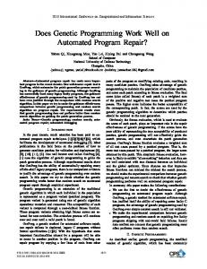
Santa Fe Trail The Santa Fe trail problem [Langdon and Poli, 1998], also known as the artificial ant problem develops a program to guide an ant along a path of food. Along this path, food becomes less frequent. The environment is modeled as
6
Figure 1.1. Santa Fe Trail Problem
a 32 by 32 discrete toroid which allows the ant to wrap from the left side to the right side of the landscape as well as from the bottom to the top. The ant starts in the Northwest corner facing east. The program is repeated until either all the food has been eaten or 500 non-terminal actions have been performed. The fitness measure of a program is the percentage of food along this trail that is eaten. The complete trail is shown in figure 1.1.
Intertwined Spirals The intertwined spirals problem [Koza, 1992a] is a classification problem. The goal is to evolve a program that correctly determines which of two spirals a given point is on. The points used include 96 points from each spiral. Figure 1.2 shows the points used. The fitness measure for a solution is what percentage of the 192 points are classified correctly. Because the classification requires a Boolean value, but the calculations use floating point numbers, the value produced by an individual is compared to 0. Values greater than or equal to zero are considered to be classified on the first spiral, and values less than zero are classified on the second spiral. The constants used for this problem are created uniformly on the interval −1.0 to 1.0. The division operator returns 1.0 when the divisor’s magnitude is less than 0.000001.
1.0
Does Genetic Programming Inherently Adopt Structured Design Techniques?
●
7
● ● ●
●
●
●
●
● ●
0.5
●
●
●
●
●
●
●
●
● ●
●
●
● ●●●●● ●● ● ● ● ● ● ● ● ● ● ●
●
y
● ●
●
●
●
● ●
●
●
●
● ●
●
●
● ●
●
● ● ● ●
●
● ●
●
●
●
●
−0.5
●
●
●
●
●
0.0
● ●
●
●
●
●
● ●
● ● ●
●
●
●
●
● ● ● ● ● ●
●
−1.0
●
−0.5
0.0
0.5
x
Figure 1.2. Intertwined Spirals Problem
Symbolic Regression Symbolic regression attempts to evolve a function that approximates a group of sampled points. For this experiment, the sampled points are taken from the function sin(x) at intervals of 0.5 starting at 0. These points are shown in Figure 1.3. This simple regression function was chosen to simplify the problem which has many operators and tends to be ‘difficult’. The error measurement used is simply the sum of the residuals between the actual points and the function evolved. In order to scale this error to the common 0.0 to 1.0 scale, the fitness function was 0.933error . The constant 0.933 was chosen to give a fitness of 0.5 when the evaluation function had an average error of 1.0 per point. The constants used in this problem are generated uniformly on the interval -2.0 to 2.0. The division operator is protected in the same way as with the Santa Fe Trail problem.
Even Parity The 6 bit even parity problem tries to evolve a Boolean function that returns the even parity of 6 input bits. The fitness of each individual is calculated by trying all 64 possible input configurations. The fitness is the percentage of these that give the correct output bit.
1.0
8
● ● ●
0.5
● ●
0.0
sin(x)
●
●
−0.5
●
−1.0
●
●
0
1
2
3
4
5
x
Figure 1.3. Symbolic Regression Problem
Battleship This chapter introduces the battleship problem. This problem was designed to be similar to the Santa Fe Trail problem, but it was hoped that the different states or behaviors would allow more opportunity for design. The problem is based on the Battleship board game with only one player. The game is played on a 10 by 10 grid which contains one ship of length 5, one of length 4, two of length 3, and one of length 2. Figure 1.4 shows an example layout of ships. The goal is to hit the ships by moving a target over their location and firing. The target starts in the Northeast corner. The landscape does not wrap around from the left to right or top to bottom. A program is allowed up to 500 operations and up to 70 shots per game. In order to calculate the fitness of a solution, 25 games are played. The fitness is the total number of hits divided by the total number of possible hits. The 25 boards are created randomly and are not changed between generations. The terminals for this problem are North, East, South, West, and No-Op. The first four move the target in the indicated direction one step. No-Op leaves the target unchanged. All 5 terminals count toward the 500 step limit. The nonterminals for this problem are Fire, Prog2, and Loop. Fire conditionally executes either the left or the right branch based on whether there is a ship at the target location. This nonterminal counts toward the 70 shot limit and
Does Genetic Programming Inherently Adopt Structured Design Techniques?
9
Figure 1.4. Battleship Problem
if there is a ship at the current target location, it is hit. Prog2 unconditionally executes its left and then its right branch. Loop is an unconditional loop that terminates only when the loop has no effect or the step limit is reached. For example if the only child of a Loop nonterminal is a West terminal, then the target would move all the way to the left of the board. Once there, the West terminal no longer has an effect and the loop terminates.
3.
Results
Table 1.1 shows the average finesses for each of the functions for each problem. The fixed root design that averaged the best fitness for each of the test problems is shown in bold. For example, the best results for the Santa Fe Trail problem occur when the root is fixed as Prog2. In general, the differences in fitness are not statistically significant or, if significant, are fairly minor. This suggests that GP can easily adapt to whatever non-terminal is fixed at the root node. Table 1.2 shows the results from the second experiment. This table shows the percentage of populations which converged to each nonterminal and the resulting average fitness and standard deviation (in parentheses). For reference, the values corresponding to the best design found in the first experiment are shown in bold. For example, with the Santa Fe Trail problem, in 42% of the
10 Table 1.1. The fixed root node that produced the best results for each of the test problems.
Santa Fe Trail
Intertwined Spirals
Symbolic Regression
Even Parity
Battleship
Design IfFood Prog2 Prog3 Plus Minus Times Divide Compare Sin Cos Plus Minus Times Divide And Nand Or Xor Fire Prog2 Loop
Fitness 0.6900 (0.1192) 0.7162 (0.1360) 0.7013 (0.1285) 0.6548 (0.03569) 0.6553 (0.03585) 0.6616 (0.03708) 0.6602 (0.03507) 0.6797 (0.03445) 0.6625 (0.04675) 0.6542 (0.04012) 0.9251 (0.02930) 0.9247 (0.03324) 0.9390 (0.02754) 0.9289 (0.04676) 0.9661 (0.07339) 0.9403 (0.08370) 0.9618 (0.07272) 0.9907 (0.03135) 0.7259 (0.1174) 0.7726 (0.06443) 0.7461 (0.09946)
1000 trials the population converged on the IfFood nonterminal as a root node and in those trials the average best fitness was 0.6866. These results show that the design/root node choice makes a small, but significant, difference in the final fitness. Comparison of the best and worst root node choices shows a significant difference in all of the problems. In four of the five problems the best non-terminal selected via experiment one also produced the best fitness in experiment two. (The exception was the even parity problem where Xor is the best non-terminal with fixed root nodes, but Nand performed better as an evolved root node.) Thus, although the fitness differences seen in experiments 1 and 2 are small, the results are consistent between the fixed and evolved cases. This supports the idea that for these problems there is a good design and a bad design as represented by the root node non-terminal. However, it is also clear that GP does not always select the optimal root node. In only two problems (parity and battleship) was the ‘best’ non-terminal, as determined in the first experiment, clearly favored by the GP and in only one case (battleship) did the favored non-terminal produce the best results. (Strictly speaking the favored
Does Genetic Programming Inherently Adopt Structured Design Techniques?
11
Table 1.2. Evolved Designs for Each Test Problem
Santa Fe Trail
Intertwined Spirals
Symbolic Regression
Even Parity
Battleship
Converged Root IfFood Prog2 Prog3 Unconverged Plus Minus Times Divide Compare Sin Cos Unconverged Plus Minus Times Divide Unconverged And Nand Or Xor Unconverged Fire Prog2 Loop Unconverged
Evolved Fitness 0.6866 (0.1159) 0.7163 (0.1300) 0.7115 (0.1259) 0.6899 (0.1366) 0.6539 (0.03637) 0.6566 (0.02821) 0.6638 (0.03450) 0.6726 (0.03641) 0.6812 (0.03499) 0.6729 (0.04009) 0.6485 (0.03580) 0.6539 0.9297 (0.02782) 0.9287 (0.02836) 0.9410 (0.02793) 0.9364 (0.04157) 0.9251 (0.04460) 0.9420 (0.08743) 0.9913 (0.03199) 0.9815 (0.04180) 0.9871 (0.03653) 0.9954 (0.02280) 0.6591 (0.1074) 0.7685 (0.06788) 0.7530 (0.08361) 0.7840 (0.05223)
% of Trials 42% 34% 23% 1.5% 17% 15% 15% 14% 18% 13% 5% 3% 12% 11% 30% 46% 2% 10% 7% 3% 73% 7% 5% 82% 6% 7%
non-terminal for intertwined spirals, Compare, also produced the best results, but it was favored by such a small margin that the results are not conclusive.) With both even parity and battleship an argument that GP adopts a topdown design methodology could be made. In both cases the non-terminal that produced the best results when fixed is heavily favored and produces the best or nearly the best results when allowed to evolve. For these problems the evolutionary process appears to be recognizing and applying a beneficial design in the majority of trials. However, for the other problems this is not the case, instead the GP settles on a non-terminal that does not generate the best results when fixed or when evolved (e.g. for the Santa Fe Trail the GP settles on the IfFood root in the majority of trials even though Prog2 and Prog3 both produce better results on average, Table 1.2).
12 Table 1.3. Initial Fitness for Each Operator for Each Problem
Santa Fe Trail
Intertwined Spirals
Symbolic Regression
Even Parity
Battleship
Root Design IfFood Prog2 Prog3 Plus Minus Times Divide Compare Sin Cos Plus Minus Times Divide And Nand Or Xor Fire Prog2 Loop
Best Initial 0.3089 (0.07572) 0.3011 (0.07780) 0.2886 (0.06271) 0.5548 (0.01445) 0.5556 (0.01606) 0.5557 (0.01419) 0.5577 (0.01702) 0.5557 (0.01460) 0.5617 (0.01826) 0.5604 (0.01576) 0.7179 (0.05078) 0.7100 (0.04861) 0.6912 (0.03689) 0.6883 (0.02609) 0.5754 (0.03314) 0.5776 (0.02904) 0.5728 (0.03246) 0.5873 (0.03821) 0.2197 (0.05904) 0.2452 (0.07965) 0.2294 (0.05984)
% of Trials 30% 35% 35% 16% 15% 16% 16% 14% 18% 5% 10% 15% 32% 42% 18% 16% 14% 53% 27% 52% 21%
Our third experiment was designed to determine how GP selects the root nonterminal, given that it does not appear to select the non-terminal that results in the best solution. We hypothesize that GP either selects the non-terminal that produces the best overall fitness in the initial population or that GP selects the non-terminal that is most frequently the root node of the best individual in the initial population. To test these hypotheses we examine the frequency with which a particular non-terminal produces the best of population member when that function is the root node and the average fitness of the best of population members with that function as the root node. Table 1.3 shows how frequently each non-terminal is the root node of the best individual in the initial random populations and the average fitness of the best individuals with each non-terminal as the root node. E.g. for the Santa Fe Trail, in the initial population the best individual had the root node Prog2 in 35% of the trials and the average fitness of the best individuals from those 35% of the trials was 0.3011. The best design, as determined by the first experiment, is emphasized in bold. The results suggest that both overall best fitness and frequency of best fitness are important. Table 1.3 shows that for both even-parity and battleship (the two
Does Genetic Programming Inherently Adopt Structured Design Techniques?
13
problems that seemed to adopt the best design) over half of the best individuals in the initial populations used the best top-level design, as determined by the first experiment, and that those individuals had the highest average fitness. The Santa Fe Trail, intertwined spirals, and symbolic regression problems the function producing the best fitness in the initial population is different from the function that most often produces the best fitness. For example, among the best programs for symbolic regression in the 1000 initial populations the programs with IfFood as the root node have the highest average fitness, but programs with Prog2 as the root are more likely to have the highest fitness. Also, for these three problems, the node leading to the greatest number of best of population programs is much less clearly defined. Table 1.4. Design Evolution for Santa Fe Trail
Final Design IfFood Prog2 Prog3
IfFood 70% 28% 31%
Prog2 15% 55% 31%
Prog3 14% 16% 36%
Table 1.5. Design Evolution for Intertwined Spirals
Final Design Plus Minus Mul Div Cmp Sin Cos
Plus 57% 10% 9% 6% 8% 15% 12%
Minus 8% 57% 8% 9% 9% 6% 4%
Mul 6% 6% 56% 13% 6% 4% 2%
Div 7% 6% 7% 52% 4% 7% 4%
Cmp 10% 10% 9% 9% 66% 11% 10%
Sin 4% 8% 4% 5% 4% 52 2%
Cos 3% 1% 2% 0% 2% 1% 66%
Tables 1.4-1.8 show a more detailed breakdown of the results of the third experiment. Each row in these tables shows the distribution of final designs given the initial design of the population. For example, in table 1.4, the first row of data shows that with the Santa Fe Trail problem in the initial populations where IfFood is the design of the best individual, 70% of the populations converged to IfFood designs, 15% to Prog2 designs, and 14% to Prog3 designs. Thus, for the Santa Fe Trail, the root non-terminal of the best individual in the initial population is significant in determining the converged root non-terminal after 100 generations.
14 Table 1.6. Design Evolution for Symbolic Regression
Final Design Plus Minus Times Divide
Plus 33% 9% 10% 9%
Minus 8% 29% 10% 7%
Times 22% 25% 43% 22%
Divide 36% 34% 35% 60%
Table 1.7. Design Evolution for Even Parity
Final Design And Nand Or Xor
And 28% 7% 4% 6%
Nand 6% 19% 6% 4%
Or 0% 2% 10% 2%
Xor 54% 65% 70% 83%
Table 1.8. Design Evolution for Battleship
Final Design Fire Prog2 Loop
Fire 9% 3% 5%
Prog2 79% 87% 73%
Loop 4% 5% 12%
In each table, the column which represents the best final design (from experiment 1) has been emphasized in bold. In most cases the function that (as the root node) generated the best of population individual in the initial population is the root node that the population converges to by the final generation. One exception is Minus in the symbolic regression problem. In the trials where Minus was the root node of the best individual 34% of the populations converged on Divide as the root node function and only 25% populations maintained Minus as the root node function. These results suggest that in most cases the root node converges on a nonterminal before sampling sufficient individuals to identify the optimal design/nonterminal. This is mostly clearly shown for the Intertwined Spirals problem, table 1.5. Along the diagonal where the initial best design matches the final design, all the values are over 50%. This implies that in over 50% of the trials, the final design is determined by the best individual in the initial random pop-
Does Genetic Programming Inherently Adopt Structured Design Techniques?
15
ulation. This could be viewed as premature convergence. With Even parity, Xor seems sufficiently better than the other operators that it attracts from other designs. However, there is still a small ‘trap’ for the other operators. For example 28% of the time when And is the design of the best individual in the initial population, it is also the final design that is converged to. The percentages of Nand and Or are smaller. The same appears true for the battleship problem. The ‘designs’ of the Santa Fe Trail, intertwined spirals, and symbolic regression problems are misleading. Table 1.3 shows that in all three problems the optimal root node function from the first experiment appears as the optimal root node function in less than half of the trials. In addition, in the cases of the intertwined spirals and symbolic regression problems, other designs appeared more frequently than the optimal designs. The data for Santa Fe Trail is less clear. It appears that there are several ‘traps’ with the initial design. If the initial best design is IfFood, 70% of the populations will evolve with the same design. With Prog2, the best design, only 55% of the populations will evolve to the same design. If the initial best design is Prog3, the final designs appear to be randomly distributed. For Symbolic Regression, Divide seems to trap and Plus and Minus seem to be redistributed. It is also interesting that different designs rarely result in a Plus or Minus in the final design. So, there is some ‘design’ away from specific non-terminals.
4.
Discussion and Conclusions
Genetic programming appears to mimic top-down design methods in that it fixes programs from the root, which solves the broadest problem, down, thereby dividing each problem into two (or more) sub-problems. GP also settles on a general program structure early in the evolutionary process. However, the root non-terminal appears to be chosen largely based on the results of the first generation. This works well when the best initial non-terminal root is the overall best choice. However, many problems appear to be deceptive; the non-terminal that produces the best results in the initial population does not lead to the best results. For other problems there is no clear favorite in the initial population and the favored non-terminal root node arises by chance. In both of these cases the fixing of the root node can be viewed as an example of partial premature convergence; the population converges on a particular nonterminal for the root node without sufficient exploration to determine if that is the ideal root node. However, unlike a GA where prematurely fixing a bit can have significant affects on fitness, GP appears to be fairly adept at finding a near optimal solution even when a poor choice is made for the root node. Given that genetic programming appears to be converging on the top-level nodes too quickly, at least for the more difficult and deceptive problems, there are several methods that may be useful to improve performance. Increasing
16 the population size may allow the evolutionary process to sample enough individuals that the best design is more likely to be chosen. However, if design complexity were to increase linearly, it is expected that the population size would need to increase exponentially to be as effective. Another possibility would be to apply fitness sharing using the design of each individual. This would reduce the convergence problem, but would become more expensive and less reliable as the depth of the design considered increases. Manually forcing the root node to a predetermined best non-terminal would not improve performance very much (average fitness for experiments 1 and 2). In general, at least for these problems the difference in fitness between optimal and non-optimal root functions did not have a large effect on performance.
References
Angeline, P. J. and Pollack, J. B. (1993). Evolutionary module acquisition. In Fogel, D. and Atmar, W., editors, Proceedings of the Second Annual Conference on Evolutionary Programming, pages 154–163, La Jolla, CA, USA. Burke, Edmund, Gustafson, Steven, and Kendall, Graham (2002). A survey and analysis of diversity measures in genetic programming. In Langdon, W. B., Cant´u-Paz, E., Mathias, K., Roy, R., Davis, D., Poli, R., Balakrishnan, K., Honavar, V., Rudolph, G., Wegener, J., Bull, L., Potter, M. A., Schultz, A. C., Miller, J. F., Burke, E., and Jonoska, N., editors, GECCO 2002: Proceedings of the Genetic and Evolutionary Computation Conference, pages 716–723, New York. Morgan Kaufmann Publishers. Daida, Jason M. (2003). What makes a problem GP-hard? In Riolo, Rick L. and Worzel, Bill, editors, Genetic Programming Theory and Practice, chapter 7, pages 99–118. Kluwer. Daida, Jason M., Hilss, Adam M., Ward, David J., and Long, Stephen L. (2003). Visualizing tree structures in genetic programming. In Cant´u-Paz, E., Foster, J. A., Deb, K., Davis, D., Roy, R., O’Reilly, U.-M., Beyer, H.-G., Standish, R., Kendall, G., Wilson, S., Harman, M., Wegener, J., Dasgupta, D., Potter, M. A., Schultz, A. C., Dowsland, K., Jonoska, N., and Miller, J., editors, Genetic and Evolutionary Computation – GECCO-2003, volume 2724 of LNCS, pages 1652–1664, Chicago. Springer-Verlag. Koza, John R. (1992a). A genetic approach to the truck backer upper problem and the inter-twined spiral problem. In Proceedings of IJCNN International Joint Conference on Neural Networks, volume IV, pages 310–318. IEEE Press. Koza, John R. (1992b). Genetic Programming: On the Programming of Computers by Means of Natural Selection. MIT Press, Cambridge, MA, USA. Koza, John R. (1994). Genetic Programming II: Automatic Discovery of Reusable Programs. MIT Press, Cambridge Massachusetts. Lambert, Kenneth A., Nance, Douglas W., and Naps, Thomas L. (1997). Introduction to Computer Science with C++. PWS Publishing Company, Boston, MA, USA.
18 Langdon, W. B. (2000). Quadratic bloat in genetic programming. In Whitley, Darrell, Goldberg, David, Cantu-Paz, Erick, Spector, Lee, Parmee, Ian, and Beyer, Hans-Georg, editors, Proceedings of the Genetic and Evolutionary Computation Conference (GECCO-2000), pages 451–458, Las Vegas, Nevada, USA. Morgan Kaufmann. Langdon, W. B. and Poli, R. (1998). Why ants are hard. In Koza, John R., Banzhaf, Wolfgang, Chellapilla, Kumar, Deb, Kalyanmoy, Dorigo, Marco, Fogel, David B., Garzon, Max H., Goldberg, David E., Iba, Hitoshi, and Riolo, Rick, editors, Genetic Programming 1998: Proceedings of the Third Annual Conference, pages 193–201, University of Wisconsin, Madison, Wisconsin, USA. Morgan Kaufmann. Langdon, William B., Soule, Terry, Poli, Riccardo, and Foster, James A. (1999). The evolution of size and shape. In Spector, Lee, Langdon, William B., O’Reilly, Una-May, and Angeline, Peter J., editors, Advances in Genetic Programming 3, chapter 8, pages 163–190. MIT Press, Cambridge, MA, USA. McPhee, Nicholas Freitag and Hopper, Nicholas J. (1999). Analysis of genetic diversity through population history. In Banzhaf, Wolfgang, Daida, Jason, Eiben, Agoston E., Garzon, Max H., Honavar, Vasant, Jakiela, Mark, and Smith, Robert E., editors, Proceedings of the Genetic and Evolutionary Computation Conference, volume 2, pages 1112–1120, Orlando, Florida, USA. Morgan Kaufmann. Rosca, Justinian (1995). Towards automatic discovery of building blocks in genetic programming. In Siegel, E. V. and Koza, J. R., editors, Working Notes for the AAAI Symposium on Genetic Programming, pages 78–85, MIT, Cambridge, MA, USA. AAAI. Rosca, Justinian P. and Ballard, Dana H. (1996). Discovery of subroutines in genetic programming. In Angeline, Peter J. and Kinnear, Jr., K. E., editors, Advances in Genetic Programming 2, chapter 9, pages 177–202. MIT Press, Cambridge, MA, USA. Soule, Terence and Foster, James A. (1998). Removal bias: a new cause of code growth in tree based evolutionary programming. In 1998 IEEE International Conference on Evolutionary Computation, pages 781–186, Anchorage, Alaska, USA. IEEE Press.