The integration of production data in to reservoir modeling is usually ac- complished through computer simulation. Normally, multiple simulations are conducted ...
Chapter 12 APPLYING GENETIC PROGRAMMING TO RESERVOIR HISTORY MATCHING PROBLEM Tina Yu^, Dave Wilkinson^ and Alexandre Castellini^ 1
2
Memorial University of Newfoundland, St. John's, NLAIB 3X5, Canada; Chevron Energy Technology Company, San Ramon, CA 94583 USA. Abstract
History matching is the process of updating a petroleum reservoir model using production data. It is a required step before a reservoir model is accepted for forecasting production. The process is normally carried out by flow simulation, which is very time-consuming. As a result, only a small number of simulation runs are conducted and the history matching results are normally unsatisfactory. In this work, we introduce a methodology using genetic programming (GP) to construct a proxy for reservoir simulator. Acting as a surrogate for the computer simulator, the "cheap" GP proxy can evaluate a large number (millions) of reservoir models within a very short time frame. Collectively, the identified goodmatching reservoir models provide us with comprehensive information about the reservoir. Moreover, we can use these models to forecast future production, which is closer to the reality than the forecasts derived from a small number of computer simulation runs. We have applied the proposed technique to a West African oil field that has complex geology. The results show that GP is able to deliver high quality proxies. Meanwhile, important information about the reservoirs was revealed from the study. Overall, the project has successfully achieved the goal of improving the quality of history matuching results without increasing the number of reservoir simulation runs. This result suggests this novel history matching approach might be effective for other reservoirs with complex geology or a significant amount of production data.
Keywords:
reservoir modeling, history matching, flow simulator, proxy, surrogate model, production forecast, uncertainty, response surface, meta-models, uniform design, experimental design
188
1.
GENETIC PROGRAMMING THEORY AND PRACTICE IV
Introduction
Petroleum reservoirs are normally large and geologically complex. In order to make management decisions that maximize oil recovery, reservoir models are constructed with as many details as possible. Two types of data that are commonly used in reservoir modeling are geophysical data and production data. Geophysical data, such as seismic and wire-line logs, describe earth properties, e.g. porosity, of the reservoir. In contrast, production data, such as water and oil saturations and pressure information, relate to the fluid flow dynamics of the reservoir. Both data types are required to be honored so that the resulting models are as close to reality as possible. Based on these models, managers make business decisions that attempt to minimize risk and maximize profits. The integration of production data in to reservoir modeling is usually accomplished through computer simulation. Normally, multiple simulations are conducted to identify reservoir models that generate fluid dynamics matching the production data collected from the field. This process is called history matching. History matching is a challenging task for the following reasons: • Computer simulation is very time consuming. On average, each run takes 2 to 10 hours to complete. • This is an inverse problem where more than one reservoir model can produce flow outputs that give acceptable match to the production data. As a result, intensive research has been devoted to making the history matching process more efficient and to delivering quality results. In this chapter, we introduce a methodology incorporating genetic programming (GP) (Koza, 1992; Banzhaf et al., 1998) to improve the history matching process. We start by explaining the reservoir history matching problem and reviewing related works in Section 2 . The methodology is then presented in Section 3. After that, we report a case study using the developed methodology and present the results in Section 4. Finally, we conclude the chapter and outline our future work in Section 5.
2.
Reservoir History Matching Problem
When an oil field is first discovered, the reservoir model is initially constructed using geophysical data. This is a forward modeling task and can be accomplished using statistical techniques (Deutsch, 2002) or soft computing methods (Yu et al., 2003). Once the field enters into production stage, many changes take place in the reservoir. For example, the extraction of oil/gas/water from the field can cause the fluid pressures of the field to change. In order to obtain the most current state of a reservoir, these changes need to be reflected in the model. History matching is the process of updating reservoir descriptor
Applying Genetic Programming to Reservoir History Matching Problem
189
Transmissibillty? Permeability?
Water rate
^^^^^^ *^^^^^^^| ^mmifll
—• Oil rate ». Bottom Hole Pressure
Reservoir Model
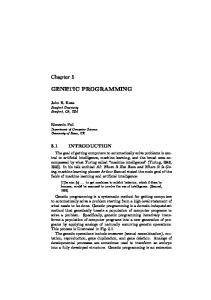
Figure 12-1. History matching is an inverse problem.
parameters to reflect such changes, based on production data collected from the field. Using the updated models, petroleum engineers can make more accurate production forecasts. The results of history matching and subsequent production forecasting strongly impact reservoir management decisions. History matching is an inverse problem. In this problem, a reservoir model is a black box with unknown parameters values (see Figure 12-1). Given the water/oil rates and other production information collected from the field, the task is to identify these unknown parameter values such that the reservoir gives flow outputs matching production data. Since inverse problems have no unique solutions, i.e. more than one combination of reservoir parameter values give the same flow outputs, we need to obtain a large number of well-matched reservoir models in order to achieve high confidence of the history-matching results. Figure 12-2 depicts the work flow of history matching and production forecast process. Initially, a base geological model is provided. Next, parameters which are believed to have impact on the reservoir fluid flow are selected. Based on their knowledge about the field, geologists and petroleum engineers then determine the possible value ranges of these parameters and use these value to conduct computer simulation runs. A computer reservoir simulator is a program which consists of mathematical equations that describe fluid dynamics of a reservoir under different conditions. The simulator takes a set of reservoir parameter values as inputs and returns a set of fluid flow information as outputs. The outputs are usually a time-series over a specified period of time. That time-series is then compared with the historical production data to evaluate their match. If the match is not satisfactory, experts would modify the parameter values and make a new simulation run. This process continues until a satisfactory match between simulation flow outputs and the production data is reached. This manual process of history matching is subjective and labor-intensive, because reservoir parameters are adjusted one-at-a-time to refine the simulations. Meanwhile, the goodness of the matching results depends largely on the experience of the team members involved in the study. Consequently, the reliability of the forecasting is often very short-lived, and the business decisions made may have a large degree of uncertainty.
190
GENETIC PROGRAMMING THEORY AND PRACTICE IV
Geological model created with static data
History matching
Design reservoir parameters to m a k e simulation runs
Select models whose simulation outputs that best match production data
Forecast with uncertainty
from Jorge Landa, Chevron (2003)
Figure 12-2. Reservoir history matching and production forecasting work flow.
To improve the quality of history matching results, several approaches have been proposed to assist the process. For example, gradient-based algorithms have been used to select sampling points sequentially for further computer simulations (Bissell et al., 1994). Although this approach can quickly find models that match production data, it may cause the search to become trapped in a local optimum and prevent models with better matches being discovered. Another shortcoming is that the method generates a single solution, despite the fact that multiple models can match the production data equally well. To overcome these issues, genetic algorithms have been proposed to replace gradient-based algorithms (Wen et al., 2004; Yu et al., 2006a). Although the results are significantly better, the computation time is not practical for large reservoir fields. There are also several works that construct a response surface that reproduces the approximate reservoir simulation outcomes. The response surface is then used as a surrogate or proxy for the costly full simulator (Narayanan et al., 1999). In this way, a large number of reservoir models can be sampled within a short period of time. Response surfaces are normally polynomial function. Recently, Kriging interpolation and neural networks have also been used as alternative methods (Yeten et al., 2005; Castellini et al., 2004). The response surface approach is usually carried out in conjunction with experimental design, which selects sample points for computer simulation runs (Eidi et al., 1994). Ideally, these
Applying Genetic Programming to Reservoir History Matching Problem
191
uniform V
li ^
o
F *
o
o
o
^
1 11
a
o— ©
0
o
1
'^^ 1 d o 1
parameter 1
Figure 12-3. Uniform sampling gives good coverage of the parameter space.
limited number of simulation runs would obtain the most information about the reservoir. Using these simulation data to construct a proxy, it is hoped that the proxy will generate outcomes that are close to the outcomes of the full simulator. This combination of response surface estimation and experimental design is shown to give good results when the reservoir models are simple and the amount of production data is small, i.e. the oil field is relatively young (Landa and Guyaguler, 2003). However, when the field has a complex geologic deposition or is in production for many years, this approach is less likely to produce a quality proxy (Landa et al., 2005). Consequently, the generated reservoir models contain a large degree of uncertainty.
3.
A Genetic Programming Solution
To improve the confidence of the uncertainty ranges of the reservoir models generated from history matching, we need to sample a dense distribution of reservoir models in the parameter space. Additionally, we need to know which of these models is a good match to the production data. With this information, we will be able to use the "good" models to forecast future production with a higher degree of confidence. To achieve that goal, we have adopted uniform sampling to conduct computer simulation runs and applied genetic programming for proxy construction. Uniform sampling, developed by Fang (Fang, 1980), generates a sampling distribution that covers the entire parameter space for a pre-determined number of runs (see Figure 12-3). It ensures that no large regions of the parameter space are left under sampled. Such coverage is important to construct a robust proxy that is able to interpolate all intermediate points in the parameter space. Using the simulation results, we then apply GP symbolic regression to construct a proxy. Unlike other research works where the proxy is constructed to give the same type of output as the full simulator, this GP proxy only labels a reservoir model as a good match or bad match to the production data, according
192
GENETIC PROGRAMMING THEORY AND PRACTICE IV
\ Figure 12-4. The studied oil field.
to the criterion decided by field engineers. In other words, it functions as a classifier to separate "good" models from "bad" ones in the parameter space. The actual amount of fluid produced by the sampled reservoirs is not estimated. This is a different kind of learning problem and it will be shown that GP is able to learn the task very well. After the GP classifier is constructed, it is then used to sample a dense distribution of reservoir models in the parameter space (millions of reservoir models). Those that are labeled as "good" are then studied and analyzed to identify their associated characteristics. Additionally, we will use these "good" models to forecast future production. Since the forecast is based on a large number of good models, the results are considered more accurate and closer to reality than those based on a limited number of simulation runs.
4.
A Case Study
The oil field we studied is a complex, clastic channel, reservoir situated offshore Africa. The primary reservoirs are sandstones deposited in a channelized system and have been in production since 1998. For history matching purposes, computer simulations on 4 blocks (A, B, C, D) of the area were conducted (see Figure 12-4). The reservoir parameters and their value ranges used to conduct the simulations are listed in Table 12-1. The 6 multiplier parameters are in log 10 values, while the other 4 parameters are in normal scale. They are applied to the base values in each grid of the reservoir field during computer simulation. Using uniform design to select parameter values, we conducted 1000 computer simulation runs. Among them, 894 were successful while the other 106 runs did not make to the end of the run due to system failures. Each successful run produces 3 types of fluid flow data: water rate (WR), oil rate (OR) and bottom hole pressure (BHP), between the years 1998 to 2004.
Applying Genetic Programming to Reservoir History Matching Problem
193
Table 12-1. Reservoir parameters and value ranges for computer simulation. Parameters
Min
Max
Parameters
Min
Max
KRWJ^ KRW_B KRW.C KRWJD XPERM Multiplier
0.3 0.1 0.1 0.1 1
0.7 0.5 0.5 0,5 2
ZPERM_A Multiplier ZPERM3 Multiplier ZPERM.C Multiplier ZPERM JD Multiplier FAULT_A_B Multiplier
0.01 0.01 0.01 0.01 0.0001
1 1 1 1 1
The simulation outputs from each run were compared with the production data collected from the field. The "error", defined as the mismatch between the two, is the sum squared difference which is calculated as follows: 2004
E=
Y^
{WR.obsi-WR.simif^-{OR.obsi-OR-simif+{BHP.obsi-BHP.simif
1=1998
Here, "obs" indicates production data while "sim" indicates computer simulation outputs. The largest E that can be accepted as good match is 2.8 x 10^. Based on this criterion, 541 models were labeled as "good" models while 353 are labeled as "bad" models by a petroleum engineer.
GP Experimental Setup To conduct the GP symbolic regression, we first divided the 894 data into three groups: 298 for training, 298 for validation and 298 for blind testing. Training data are used for GP to construct the classifier while validation data is used to select thefinalclassifier. In this way, over-fitting is less likely to happen. The evaluation of the classifier is based on its performance on the blind testing data. The GP system is a commercial package that makes multiple runs (Francone, 2001). Table 12-2 lists some of the GP parameters used to train the classifiers. There are other GP parameters that are notfixedbut are selected by the software for each run. These parameters include population size, maximum program size, and crossover and mutation rates. In the first run, one set of values for these parameters was specified. When the run does not produce an improved solution for a certain number of generations, the run is terminated and a new set of parameter values is selected by the system to start a new run. The system maintains the best 50 solutions found throughout the multiple runs. When the GP system is terminated, the best classifier among the pool of 50 solutions is thefinalsolution. In this work, we let the GP system continue for 120 runs and then manually terminated the system. The fitness is based on hit rate: the percentage of the training data that are correctly classified. During tournament selection, four candidates are randomly
194
GENETIC PROGRAMMING THEORY AND PRACTICE IV Table 12-2. Some of the parameters for GP symbolic regression.
Objective
Evolve a classifier that separates good reservoir models from bad ones.
Functions Terminals Fitness Hit Rate Selection
addition;subtraction;multiplication;division;abs;data transformation The 10 reservoir parameters listed in Table 12-1 Hit rate then mean squared error The percentage of the training data that are correctly classified. Tournament (4 candidates/2 winners)
selected and paired to compete for two slots. If two candidates are tied in their hit rates, the mean squared error measurement is used to select the winners. The "tied threshold" for mean squared error measurement is 0.01% in this work. If two classifiers are tied in both their hit rates and mean squared error measurements, a winner is randomly selected from the two competitors. In this application, we made two sets of batch runs. In thefirstbatch, parsimony pressure is turned on to promote shorter classifiers. During tournament selection, the GP system selects the shorter solution to be the winner if its fitness is not worse than 1 % of its competitor. To avoid the system over protecting short solutions and sacrifice quality, we allow parsimony pressure to affect only 50% of the tournament selection. Also, we disallow parsimony pressure to have any effect during the first 3 generations when the evolution search is exploring the parameter space. In the second batch, parsimony pressure is tumed off; the evolutionary search is free to explore classifiers with arbitrarily complex structures. With this setup, we can learn how much performance can be gained by trading with complexity.
Results Table 12-3 gives the results from both batch runs. When parsimony pressure is on, the best GP classifier contains 4 parameters: KRW_C, ZPERM JD, ZPERM_A and FAULT-A-B. The classification accuracy is approximately 91 %. When parsimony pressure is off, the best GP classifier contains 8 parameters and gives a slightly higher classification accuracy of 94%. Both results are very good. From the practical point of view, simpler models are easier to understand and analyze. We therefore selected the one with 4 parameters as our final solution. Figure 12-5 gives the classification results on all 894 data in the space of the 3 most important parameters (KRW.C, ZPERM A and ZPERMJD). As shown, good models are of low ZPERMJD value while bad models are with high ZPERMJ) value. Although there are a small number of misclassification, the overall trend of good reservoir models is consistent. There are other machine learning methods which can be used to train classifiers. Among them, we tested a fuzzy classifier, a linear discriminant analysisbased classifier, a self-organized map and a support vector machine. The results
Applying Genetic Programming to Reservoir History Matching Problem
195
Table 12-3. Results of GP symbolic regression runs. Training Data Accuracy Validation Data Accuracy Testing Data Accuracy Number of Reservoir Parameters Selected
Parsimony Off
Parsimony On 91.61% 91.28% 90.94% 4
a
•
•+
94.97% 93.62% 93.29% 8
good classified as good good classified as bad bad classified as good bad classified as bad
Figure 12-5. Reservoir models classification results.
Method Fuzzy Classifier LDABased Classifier SOM SVM (radial kernel) GP
Table 12-4. Results of other learning methods. Training Data Validation Data 74.232% 63.5915% 65.3105% 100% 94.97%
71.53% 58.389% 59.0105% 91.2895% 93.62%
Testing Data 69.922% 58.695% 56.0155% 92.8125% 93.29%
are shown in Table 12-4. For this set of data, the support vector machine (SVM) gives comparable results to the GP classifier. We used a radial kernel with gamma value 0.04 for SVM learning. The SVM classifier shows a tendency of over-fitting toward training data, which is not observed in the GP classifier.
196
GENETIC PROGRAMMING THEORY AND PRACTICE IV
Interpolation and Interpretation We used the simpler classifier (with 4 parameters) to evaluate new sample points in the parameter space. For each of the 4 parameters, 21 samples were selected, evenly distributed between their minimum and maximum values. The resulting total number of samples is 21^ = 194,481. Running the GP classifier on these samples resulted in 73,135 being identified as good models while 121,346 were classified as bad models.
Figure 12-6. Good reservoir models identified by the GP proxy.
Figure 12-7. Good reservoir models identified by computer simulator.
Applying Genetic Programming to Reservoir History Matching Problem
197
Figure 12-8, The upper bound of good models in the parameter space.
Figure 12-6 shows the 73,135 good models in the parameter space. They are located in the bottom half, where the ZPERMX) value is less than -0.6. This is consistent with the results of computer simulation (Figure 12-7). Also, good models in both Figures show a consistent trend of decreasing ZPERMX) value when both KRW.C and ZPERM_A increase. Another characteristic of good models is that very few of them have a FAULT_A-B value of zero (diamond shape in Figure 12-7 and 12-6). This indicates that the faults separating geobody A field and B field are not completely sealing. With these sampling results, we can draw an upper bound for good models in the parameter space (see Figure 12-8). Bad models identified by the GP classifier are shown in Figure 12-9. They occupy most parts of the parameter space, except two significant areas. One is on the left lower comer where KRW.C is less than 0.18, ZPERM A is between -2 and -0.2 and ZPERMD is between -2 and -1.1 (see Figure 12-11). The other is on the comer where ZPERM A is 0, KRW.C is less than 0.18 and ZPERMD is between -0.5 and -1.9 (see Figure 12-12 ). The bad model area identified by GP classifier covers all the bad models resulting from computer simulation (shown in Figure 12-10 ). Additionally, it also identifies that FAULT A _B zero value models are bad in the lower half of the parameter space, shown in diamond shape. Figure 12-11 and 12-12 give the lower bound of the bad models in the parameter space.
GENETIC PROGRAMMING THEORY AND PRACTICE IV
198
MMiMiUMMMMi
Figure 12-9. Bad reservoir models identified by the GP proxy. : •
Fault_A_B non-zero Falut A B zero
-_ :
i
^
'S\lt:\
^^x4^>/"4v?^#.r^t'-•r.:
Figure 12-10. Bad reservoir models identified by computer simulator.
Project Contributions Based on the history matching results, which were obtained using the developed framework and proposed techniques of uniform design and GP, we delivered the following information to the reservoir engineers. • The most important 4 parameters that influence match to the production data. •
The ranges of values for these 4 parameters that give good match to production data.
Applying Genetic Programming to Reservoir History Matching Problem
Figure 12-11, Lower bound of bad models.
199
Figure 12-12. Lower bound of bad models.
The boundary of good and bad models in the parameter space.
•
Insights in the geological compartmentalization of the reservoir.
These results are well received and verified by the field reservoir engineers. Overall, the project has successfully achieved the goal of improving the quality of the reservoir models by history matching, without increasing the number of computer simulations. This result suggests that this novel method might be effective for other reservoirs with complex geology or significant amounts of production data.
5.
Concluding Remarks
Reservoir history matching and production forecasting are of great importance to the planning and operation of oil reservoir fields. Under time pressure, it is often necessary to curtail the number of computer simulation runs and make decisions based on a limited amount of information. This work proposes using GP to construct a proxy for the full computer simulator. In this way, we can replace the simulator by the proxy in order to sample a much larger number of reservoir models and, consequently, obtain more information, which in turn, it is hoped, will lead to better reservoir decisions being made. We have conducted a case study using the proposed approach. The results have shown that the proxy gives comparable performance to that of the full simulator in distinguishing between reservoir models that are close to the reality and those that are not. This is an improvement on what has reported in the literature (see Section 2). We believe there are two possible reasons for our success:
200
GENETIC PROGRAMMING THEORY AND PRACTICE IV
• The innovative idea of casting the proxy as a classifier, which changes the nature of the problem from other works using the difference between computer simulation results and production data as the response surface. • Applying genetic programming to model this response surface, which is more suitable for this task than other learning algorithms (see Section 12-3). As far as we know, this is the first time such a method has been proposed to construct a proxy for the reservoir simulator. Based on the initial encouraging results, we have conducted another study on a different oil field with a large amount of production data. In that study, we also forecast reservoir production using the good models sampled by the GP proxy. This work is reported separately in (Yu et al., 2006b).
Acknowledgment We would like to thank Iba Hitoshi and Michael Koms for their comments and suggestions.
References Banzhaf, Wolfgang, Nordin, Peter, Keller, Robert E., and Francone, Frank D. (1998). Genetic Programming -An Introduction; On the Automatic Evolution of Computer Programs and its Applications. Morgan Kaufmann, San Francisco, CA, USA. Bissell, R. C, Sharma, Y., and Killough, J. E. (1994). History matching using the method of gradients: two case studies. Paper SPE 28590, presented at the SPE Annual Technical Conference and Exhibition, New Orleans, LA, September 25-28. Castellini, Alexandre, Landa, Jorge, and Kikani, Jitendra (2004). Practical methods for uncertainty assessment offlowpredictions for reservoirs with significant history - afieldcase study. Paper A-33, presented at the 9th European Conference on the Mathematics of Oil Recovery, Cannes, France, August 30 - September 2. Deutsch, Clayton V. (2002). Geostatistical Reservoir Modeling, Oxford University Press. Eidi, A. L., Holden, L., Reiso, E., and Aanonsen, S. I. (1994). Automatic history matching by use of response surfaces and experimental design, paper presented at the Fourth European Conference on the Mathematics of Oil Recovery, Roros, Norway, June 7-10. Fang, Kai-Tai (1980). Uniform design: Application of number theory in test design. ACTA Mathematicae Applicatae Sinica,
Applying Genetic Programming to Reservoir History Matching Problem
201
Francone, Frank D. (2001). Discipulus Owner's Manual 11757 W. Ken Caryl Avenue F, PBM 512, Littleton, Colorado, 80127-3719, USA, version 3.0 draft edition. Koza, John R. (1992). Genetic Programming: On the Programming of Computers by Means of Natural Selection, MIT Press, Cambridge, MA, USA. Landa, Jorge L. and Guyaguler, Baris (2003). A methodology for history matching and the assessment of uncertainties associated withflowprediction, paper SPE 84465, presented at the SPE Annual Technical Conference and Exhibition, Denver, CO, October 5-8. Landa, Jorge L., Kalia, R. K., Nakano, A., Nomura, K., and Bashishta, P. (2005). History match and associated forecast uncertainty analysis - practical approaches using cluster computing, paper IPTC 10751, presented at The International Petroleum Technology Conference, Doha, Qatar, November 21-23. Narayanan, K., White CD., Lake, L. W., and Willis, B. J. (1999). Response methods for up-scaling heterogeneous geologic models, paper SPE 51923, presented at the SPE Reservoir Simulation Symposium, Houston, TX, February 14-17. Wen, Xian-Huan., Yu, Tina, and Lee, Seong (2004). Coupling sequential-self calibration and genetic algorithms to integrate production data in geostatistical reservoir modeling. In Proceedings of the Seventh Geostatistics Congress, pages 691-702. Yeten, Burak, Castellini, Alexandre, Guyaguler, Baris, and Chen, Wen (2005). A comparison study on experimental design and response surface methodologies, paper SPE 93347, presented at the SPE Reservoir Simulation Symposium, Houston, TX, January 31 - February 2. Yu, Tina, Wen, Xian-Huan, and Lee, Seong (2006a). A hybrid of sequentialself calibration and genetic algorithms inverse technique for geostatistical reservoir modeling. In Proceedings of the IEEE World Congress on Computational Intelligence, Yu, Tina, Wilkinson, Dave, and Castellini, Alexandre (2006b). Constructing reservoirflowsimulator proxies using genetic programming for history matching and production forecast uncertainty analysis, submitted. Yu, Tina, Wilkinson, Dave, and Xie, Deyi (2003). A hybrid GP-fuzzy approach for reservoir characterization. In Riolo, Rick L. and Worzel, Bill, editors. Genetic Programming Theory and Practise, chapter 17, pages 271 -290. Kluwer.