Chapter 11 Learning and Representation - Neural Information ...

Handbook of Large-Scale Random Networks pp. 1–484.

BOLYAI SOCIETY MATHEMATICAL STUDIES, 18

Chapter 11 Learning and Representation: From Compressive Sampling to the ‘Symbol Learning Problem’ ´ LORINCZ ˝ ANDRAS

In this paper a novel approach to neurocognitive modeling is proposed in which the central constraints are provided by the theory of reinforcement learning. In this formulation learning is (1) exploiting the statistical properties of the system’s environment, (2) constrained by biologically inspired Hebbian interactions and (3) based only on algorithms which are consistent and stable. In the resulting model some of the most enigmatic problems of artificial intelligence have to be addressed. In particular, considerations on combinatorial explosion lead to constraints on the concepts of state–action pairs: these concepts have the peculiar flavor of determinism in a partially observed and thus highly uncertain world. We will argue that these concepts of factored reinforcement learning result in an intriguing learning task that we call the symbol learning problem. For this task we sketch an information theoretic framework and point towards a possible resolution.

1. Introduction Reinforcement learning (RL) has successfully reached human level in different games [119, 15, 12, 22, 103, 26, 112, 113]. Furthermore, RL has attractive, near optimal polynomial time convergence properties under certain conditions [57, 16]. Because RL has been strongly motivated by psychology and neuroscience [101, 81, 87, 27, 94, 29, 63, 99], too, we take the Markov decision problem (MDP) model of RL as the central organization concept in

2

A. L˝ orincz

modeling the brain. It means that we have to win through the limitations arising from the Markovian assumption. The core problem of RL is that even simple agents in simple environments need a number of variables to detect, such as objects, their shape or color, other agents, including relatives, friends, and enemies, or the space itself, e.g., distance, speed, direction, and so on. The size of the state space grows exponentially in the number of the variables. The base, which corresponds to the discretization of the variables, and the number of possible actions are less harmful. However, another source of combinatorial explosion comes from partial observation; agents need to maintain a history of sensory information. This temporal depth comes as a multiplier in the exponent again. In the so-called multi-agent systems, the problem becomes even harder as the internal states of the other learning agents are hidden. This fact has serious consequences. First, the number of agents also multiplies the exponent. Second, the hidden nature of the internal states violates the central assumption of RL about the Markov property of the states. For a review on multi-agent RL, see e.g., [53, 17]. The effect of hidden variables is striking. For example, we have found that, for two agents with two hidden states (meaning) and two actions (signals to the other agent), some cost on communication is enough to prohibit an agreement on signal meaning association [71]. Nevertheless, there is a resolution if an agent can build an internal model about the other agent. In this case they can quickly come to an agreement. This situation is best described as ‘I know what you are thinking and I proceed accordingly’. However, if both agents build models about each other, then agreement is again hard, unless one of the agents assumes that the other agent also builds a model, like ‘I know that you know what I am thinking’. Such observations highlight the relevance of model construction and the adjustment of the estimated reward function by, for example, inverse reinforcement learning [83] and apprenticeship learning [1, 82]. Within the framework of RL, factored description can decrease the exponent of the state space [13, 14, 61, 44]. In the multi-agent scenario, for example, if it turns out that a given agent (let us say, agent B) does not influence the long-term goals in the actual events observed by another agent (agent A), then the variables corresponding to agent B can be dropped; only the relevant factors need to be considered by agent A at that time instant. Limitations of RL highlight the learning task that finds the relevant factors for model construction.

Learning and Representation

3

In the approach presented in this paper two different types of constraints will be applied. There is a set of experimental constraints coming from neuroscience and cognition. These should be considered as soft constraints, because the interpretation of the findings is debated in many cases. However, these constraints help to reduce the number of potential machine learning approaches. The other type of constraints comes from mathematics. These are hard constraints and are the most important supporting tools. However, care should be taken as they may have also have their own pitfalls hidden deeply in the assumptions, like the conditions of the different theorems applied. Ideally, building a model should start from a few philosophical principles, should be constrained by (1) the need for fast learning (because of the evolutionary pressure), by (2) the complexity of the environment and the tasks, and by (3) the different aspects of determinism and stochastic processes. The emerging model should then be used to derive the global structure of the brain as well as the tiniest details of the neural organization. This dream is certainly beyond our current knowledge and will stay so for a long time. Instead, a compromise is put forth here: I will start from the constraints of reinforcement learning, will consider certain facts of the environment and will build upon those in the quest for the solution. If there is some reassuring information or guideline from neuroscience then I will mention those, but the set of choices is certainly subjective. At each point we will find new sources of combinatorial explosion and will proceed in order to decrease their impact. Eventually, we will arrive at an unresolved problem that we call the symbol learning problem. We shall argue that the symbol learning problem may eliminate the enigmatic issues of the symbol grounding problem of cognition. (For the description of the symbol grounding problem, see [47] and the references therein.) Furthermore, the symbol learning problem may gain a rigorous information theoretic formulation with some indications that polynomial time algorithms can solve it under certain conditions. In the next subsection I provide an overview of the paper. It is a linear construction with loops at each step. The loops are about the arising mathematical problems and their possible resolutions. At each step, there is a large pool of potential algorithms to resolve the emerged problems and we shall select from those by looking at the soft constraints provided by experimental neuroscience.

4

A. L˝ orincz

1.1. Overview of the structure of the paper All building blocks or computational principles have neurobiological motivation that I will refer to. In Section 2 I shortly review recent advances on compressible sensing, the relevance of sparse representation and L0 norm, and the related neural architecture. In Section 3 I show how a family of non-combinatorial independent component analysis can be structured to achieve exponential gains by breaking the sensory information into independent pieces. Reassurance and problems both come from neurobiology: learning can be put into Hebbian form and the particular form provides insight into the hippocampal formation of the brain, responsible for the formation of declarative memory. However, the same formation points to the need of action-based labeling; control and factors are interlaced. Unfortunately, action-based labeling is not feasible, because the size of label space can be enormously huge. As an example, consider the concerted actions of the muscles. For 600 independent muscle groups with, for simplicity, only 2 (‘on’ or ‘off’) stages, the label space is as large as 2600 . This issue is addressed in Section 4, where the control problem is reformulated in terms of speed-field tracking inverse dynamics that can be made robust against approximation errors. In doing so we may avoid difficulties arising from kinematics and inverse kinematics. In turn, learning becomes feasible. We also review MDPs and show that the proposed robust controller scheme fits well into the RL formalism if used within the so called event-learning framework [74, 116]. In addition, we review factored RL that is also designed to help avoid other sources of combinatorial explosions. Learning in this setup is polynomial in the number of states, which can be seen as a novel result for RL. In the context of factored RL, we need to consider partially observed environments, which in turn leads to an enigmatic problem. Namely, there is a hidden, but quite influential assumption about both the states and the actions in the traditional formalism, or about the states and the desired states in the event-based formalism. The problem is that states and actions are given, that is they have a deterministic description. Such determinism apparently contradicts to the ‘great blooming, buzzing confusion’ [54] that we observe: there are so many factors that may influence a ‘given state’ that the description is either huge and the state may never occur, or it must have stochastic components. The rescuing thought is missing. We shall formulate this cornerstone of the learning problem that we call the symbol learning problem.


5

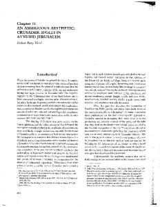
Fig. 1. Construction of the paper. Squares: facts about information from nature and algorithms. Pentagons: emergent problems that need to be solved to proceed further. Hexagons: reassuring soft information from neuroscience and cognition

2. Sparse Representation

I review certain features of perception and natural stimuli. Then I introduce the notion of sparse representation and discuss how it enables factored representation, which unfortunately still leads to combinatorial explosion. One of the most relevant problems for computational models is the maintenance of distinct interpretations of environmental inputs. The presence of competing representations is not simply a plausible assumption, but it has strong psychophysical and neurobiological support in rivalry situations, when two or more likely interpretations ‘fight’ to reach conscious observation, but our mind chooses between them and only one ‘meaning’ is present at a time [67, 65]. However, while it inhibits the conscious concurrent observation, it also enables switches among the different interpretations in a

6

A. L˝ orincz

robust manner. Switching is so robust that usually we can not prevent it at will [66, 21]. In turn, while the inputs are continuous, the existence of distinct representations point to some kind of discrete nature of the representation. It has been observed that typical signals have specific statistical properties, distributions are not Gaussian but they are heavy-tailed in many cases. This means that information is compressible in the sense that there exist bases where the representation has a few large coefficients and many small ones. This is the case, for example, for natural images. The accommodation of biological perceptual systems to such peculiar statistical properties have been extensively studied (see, e.g., [36, 32, 31]). It is also known that sparse overcomplete representation can be learned robustly in artificial neural networks for the case of natural images; properties of the emerging ‘receptive fields’ have little dependence on the sparsifying non-linearity applied during learning [42, 85, 86, 96, 64]. The reason for this property remained elusive until the recent discovery of compressive sampling. It turns out that computations in L1 and in L0 norms result in the same representation for such heavy tailed distributions [19, 33, 18]. This is the so called ‘L1 Magic’ that has received considerable attention recently in diverse fields1 . 2.1. Neural solution to distinct sparse representations The basic algorithm presented in [85] can be put into a multi-layer recurrent neural network architecture. The idea can be traced back to the eighties [8, 91] and has undergone considerable developments during the last two decades, see, e.g., [56, 93, 76]. There are many variants that can be called together as autoencoders [3, 49]. In these neural architectures, however, there is no place for competition between different representations.2 Rubinstein’s global optimization technique, the so called cross entropy method (CEM) [28] has recently been used to resolve this problem. The resolution makes use of a novel online variant [115, 73] of the original batch learning method. In addition, this online variant 1 For a comprehensive collection of papers visit the compressive sampling resources of the DSP group at Rice University: http://www.dsp.ece.rice.edu/cs/ 2 In this text, we make no difference between the notions of representation and interpretation.

7


• applies directly the L0 norm, which is robust in the neural network sense: the norm is not strict as any Lq norm (where 0 ≤ q ≤ 1) may produce similar results, and • encourages us to take a fresh look on the spike-coding versus rate coding dichotomy. The basic optimization problem of sparse representation – in a nutshell – is the following: let x ∈ Rn denote the input we want to reconstruct with a sparse representation (h ∈ Rm ) using an overcomplete basis set A ∈ Rn×m , where m À n. The corresponding optimization problem is: (1)

h∗ := arg min ξ · khkL0 + kx − AhkL2 , h

where k.kLn denotes the Ln norm, ξ is a trade-off parameter. The first term enforces low number of nonzero components, the second term minimizes the L2 -norm of the reconstruction error ε(t) = x − Ah(t). We are solving the above problem using CEM as it exploits sparsity. CEM aims to find the (approximate) solution for global optimization tasks in the following form h∗ := arg min f (h). h

where f is a general objective function. Instead of having a single candidate solution at each time step, CEM maintains a distribution g(t) of h(t) for guessing solution candidates. The efficiency of this random guess is then improved by selecting the best samples – the so called ‘elite’ – and iteratively modifying g(t) to be more peaked around the elite. It is known that, under mild regularity conditions, CEM converges with probability 1 and that, for a sufficiently large population, the global optimum is found with high probability [78]. It is also known that CEM is strikingly efficient in combinatorial optimization problems. Formally, CEM works as follows. Let g belong to a family of parameterized distributions, H . Let h(1) , . . . , h(N ) be independent samples (N is fixed beforehand) from g. For each γ ∈ R, the set of ‘elite’ samples, bγ := {h(i) | f (h(i) ) ≤ γ, 1 ≤ i ≤ N }, E © ª provides an approximation to the level set Eγ := h | f (h) ≤ γ . bγ be the distribution over the level set Eγ and E bγ , reLet Uγ and U ∗ spectively. For small γ, Uγ is peaked around h . CEM chooses g(t) that

8

A. L˝ orincz

is closest in the cross-entropy (or KL divergence) metric to the empirical bγ . The algorithm iteratively modifies γ and g to reach the distribution U optimal performance value γ ∗ = f (h∗ ). CEM uses some technical tricks. bγ by maintaining the best ρ · N samples (1 − ρ It prohibits depletion of E quantile), where ρ ∈ [0, 1] is a fixed ratio. Also, it deals with parameterized distribution families where parameters can easily be approximated from simple statistics of the elite samples. Note also that updating the distribution parameters can be too coarse, so a smoothing factor α is applied. Informally, CEM is a maximum likelihood method, without immature decisions. The conservative nature of CEM comes from its innovation, the maintenance of the elite, and that it sharpens the distribution of this elite step-by-step. Our idea is that the important component of this step-by-step sharpening of the distribution, the set of elite samples need not be stored [115, 73]. Further, sparse representation resolves the dilemma on discrete versus continuous representation: CEM can search for low-complexity (sparse) representation and within each sparse representation candidate the continuous values of the representation can be computed by (iterative) pseudoinverse computation for the allowed sparse non-zero components of h denoted by hL0 (2)

∆hL0 ∝ PL0 AT ε,

where PL0 projects to the allowed non-zero set of the components of the overcomplete representation. Equation (2) is the gradient update that follows from (1) for hL0 . In sum, sparse overcompleteness has some interesting consequences. Components or features are either present or absent and thus their presence can be detected independently. Sparseness may recast the reconstruction task as a combinatorial optimization problem for which we suggested a modification of the very efficient and simple CEM. CEM is robust, fast and essentially parallel, but requires batch access to samples. Our modification resulted in an online version that may enable one to find mapping onto real neuronal networks. Another extension is that for analog valued inputs and/or representations, we embedded the online CEM into a reconstruction network architecture that can directly calculate the reconstruction error term of the cost function through feedforward and feedback connections. (See, e.g., [76] about the potential role of such networks in real neuronal systems).


9

Another important aspect of the online CEM is that it is essentially built on the concurrent use of digital (spike-based feature selection) and analog valued coding (like the input and its representation). This particular feature may contribute to the long standing debate (see e.g. [97] and references therein) about the different neuronal coding schemes by suggesting a new computational role for spikes and maintaining rate code as well. The novel interpretation is that spikes are used to improve the probability of the compositional representation, whereas rate code is about the magnitude of the selected components. Thus, beyond the advantages of the algorithm featuring global optimization and parallel sampling in distributed networks, it might have biological significance and resolve some of the puzzles of neuronal networks. A few notes are added here. Sparse representation is promising for natural signals, because it can overcome the Nyquist noise limit [19, 33, 18], enables sparse sampling and may offer insight into the two-faceted nature of neural coding, i.e., spike-coding and rate coding. Further, the presence or absence of the elements of sparse representation – in principle – enables tabulated RL methods. However, sparse coding makes combinatorial explosion even harder, implying that additional algorithmic components are needed. An individual element of the sparse neural representation can be seen as a vector with a dimension that equals the dimension of the input: for component i of representation h the synaptic vector is the ith column of matrix A. In the next section we discuss how individual elements of the neural representation can be collected into (approximately) independent groups; thus forming (approximately) independent subspaces or ‘factors’.

3. Factored Representation In the first part of this section, I review our recent results on how to collect components so that each group is approximately statistically independent from other groups. The relevance of this section is the following: 1. For groups of statistically independent components, the influence of other groups may be neglected. Thus machine learning methods may be restricted to some of the subspaces of the grouped variables making considerable savings in the exponent of the state space.

10

A. L˝ orincz

2. Dynamical dependencies of different orders, e.g., position, momentum, and acceleration, can also be factored. 3. Sparse coding, independent component analysis (ICA) and the autoregressive family of dynamical models reviewed in this section are closely related to each other [86, 108]. 4. Cardoso’s observation that components found by ICA are entailed by single independent subspaces has received mathematical support for a limited set of distributions [108]. The observation enables effective non-combinatorial search for independent subspaces, without a priori information about the number of subspaces and their dimensions. Thus, we have a non-combinatorial algorithm that can provide combinatorial gains [89]. Independent Subspace Analysis (ISA) [20] is a generalization of ICA. ISA assumes that certain sources depend on each other, but the dependent groups of sources are independent of each other, i.e., the independent groups are multidimensional. The ISA task has been subject of extensive research [20, 123, 105, 6, 121, 52, 84, 88]. Generally, it is assumed that hidden sources are independent and identically distributed (i.i.d.) in time. Temporal independence is, however, a gross oversimplification of real sources including acoustic or biomedical data. One may try to overcome this problem by assuming that hidden processes are, e.g., autoregressive (AR) processes. Then we arrive to the AR Independent Process Analysis (AR-IPA) task [51, 90]. Another method to weaken the i.i.d. assumption is to assume moving averaging (MA). This direction is called Blind Source Deconvolution (BSD) [23], where observation is a temporal mixture of the i.i.d. components. The AR and MA models can be generalized and one may assume ARMA sources instead of i.i.d. ones. As an additional step, these models can be extended to non-stationary integrated ARMA (ARIMA) processes, which are important, e.g., for modeling economic processes [80]. In the next section we review the AR-, MA-, ARMA-, ARIMA-IPA generalizations of the ISA task, when (i) one allows for multidimensional hidden components and (ii) the dimensions of the hidden processes are not known. In the undercomplete case, when the number of ‘sensors’ is larger than the number of ‘sources’, these tasks can be solved, because they can be reduced to the ISA task.

11


3.1. Non-combinatorial independent subspace analysis The ISA task can be formalized as follows: (3)

£ ¤ x(t) = Ae(t), where e(t) = e1 (t); . . . ; eM (t) ∈ RDe , m

that is e(t) is a concatenated vector of components em (t) ∈ Rde . The total PM m dimension of the components is De = m=1 de . We assume that for a m m given m, e (t) is i.i.d. in time t, and sources e are jointly independent, i.e., I(E 1 , . . . , E M ) = 0, where I(.) denotes the mutual information of the arguments, E m (m = 1, . . . , M ) is a dm e dimensional random variable with m ≤ em ). cumulative distribution function F (em ) = Pr(E1m ≤ em 1 , . . . , Edm dm e e The dimension of the observation x is Dx . Assume that Dx > De , and A ∈ RDx ×De has rank De . Then, one may assume without any loss of generality that both the observed (x) and the hidden (e) signals are white. For example, one may apply Principal Component Analysis (PCA) as a preprocessing stage. Then the ambiguities of the ISA task are as follows [120]: sources can be determined up to permutation and up to orthogonal transformations within the subspaces. 3.1.1. ISA separation. We are to uncover the independent subspaces. Our task is to find a matrix W ∈ RDe ×Dx with orthonormal columns £ ¤ (that is WWT = I) such that y(t) = Wx(t), y(t) = y1 (t); . . . ; yM (t) , m ym = [y1m ; . . . ; ydmm ] ∈ Rde , (m = 1, . . . , M ) with the condition that the e m – are components of the related dm e dimensional random variables – i.e., Y independent. Here, yim denotes the ith coordinate of the mth estimated subspace. This task can be viewed as the minimization of the mutual information between the estimated components on the orthogonal group: (4)

¢ . ¡ JI (W) = I Y 1 , . . . , Y M .

Alternatively, because (i) the entropy of the input H(x) is constant and (ii) WWT = I, (4) is equivalent to the minimization of the following cost function: (5)

M . X ¡ m¢ H Y . JH (W) = m=1

12

A. L˝ orincz

Identities for mutual information and entropy expressions can be used to derive another equivalent cost function: e

(6)

dm M M X . X X JH,I (W) = H(Yim ) − I (Y1m , . . . , Ydm m ), e m=1 i=1

m=1

and arrive finally to the following minimization problem (7)

M X . 1 M I (Y1m , . . . , Ydm JI,I (W) = I (Y1 , . . . , YdM ) − m ), e e

m=1

where Yim (m = 1, . . . , M and i = 1, . . . dem ) denote the stochastic variable related to yim . The first term of the r.h.s. of (7) is an ICA cost function; it aims to minimize mutual information for all coordinates. The other term is a kind of anti-ICA term; it maximizes mutual information within the subspaces. One may try to apply a heuristics and to optimize (7) in the following order: (1) Start by any ‘infomax’-based ICA algorithm and minimize the first term of the r.h.s. in (7). (2) Apply only permutations on the coordinates to optimize the second term. Surprisingly, this heuristics leads to the global minimum of (4) in many cases. In other words, ICA that minimizes the first term of the r.h.s. of (7) solves the ISA task as well, apart from grouping the coordinates into subspaces. This feature was first observed by Cardoso [20]. To what extent this heuristic works is still an open issue. Nonetheless, we consider it as a ‘Separation Theorem’, because for elliptically symmetric sources and for some other distribution types one can prove that it is rigorously true [107]. (See also the results concerning local minimum points [122]). Although there is no proof for general sources yet, a number of algorithms successfully apply this heuristics [20, 105, 122, 7, 106, 2]. 3.1.2. ISA with unknown components. Another issue concerns the computation of the second term of (7), because we have to group the ICA components by means of this term. For subspaces em of known dimensions dm e , multi-dimensional entropy estimations can be applied [88], but these are computationally expensive. Other methods deal with implicit or explicit pair-wise dependency estimations [7, 122]. Interestingly, if the observations are indeed from an ICA generative model, then minimization of pair-wise dependencies is sufficient to solve the ICA task according to the DarmoisSkitovich theorem [25]. For the ISA problem, in principle, estimation of


13

pair-wise dependencies is insufficient to recover the hidden subspaces [88]. Nonetheless, such algorithms seem to work nicely in many practical cases. m A further complication arises if dimensions dm e of subspaces e are not known. Then the dimension of the entropy estimation becomes uncertain. There exist methods that also try to minimize pair-wise dependencies. A block-diagonalization method has been suggested in [122], whereas [7] makes use of kernel estimations of the mutual information.

Assume that the separation theorem is satisfied and apply ICA preprocessing. This step can be followed by the estimation of the pair-wise mutual information of the ICA coordinates. These quantities can be represented as the elements of an information adjacency graph, the vertices of the graph being the ICA coordinates. One can search for clusters of this graph and may apply different efficient approximations like Kernel Canonical Correlation Analysis [6] for the estimation of mutual information. Then variants of the Ncut algorithm [124] can be used for clustering. As a result, the mutual information within (between) cluster(s) becomes large (small). Below, we show that the ISA task can be generalized to more realistic sources. 3.1.3. ISA Generalizations. We need the following notations: Let z stand for the time-shift operation, that is (zv)(t) := v(t − 1). The N order D1 ×D2 polynomials of z over the D1 × D2 matrices are denoted as R[z]N := ª © PN r n D ×D r 1 2 . Let ∇ [z] := (I − Iz) denote the rth F[z] = n=0 Fn z , Fn ∈ R order difference operator, where I is the identity matrix, r ≥ 0, r ∈ Z. Now, we are to estimate unknown components em from observed signals x. We always assume that e takes the form like in (3) and that A ∈ RDx ×Ds is of full column rank. 1. AR-IPA: The AR generalization of the ISA task is defined by the following equations: x = As, where s is a multivariate process i.e., Pp AR(p) D ×D i s e P[z]s = Qe, Q ∈ R , and P[z] := IDs − i=1 Pi z ∈ R[z]pDs ×Ds . ¡ ¢ We assume that P[z] is stable, that is det P[η] 6= 0, for all η ∈ C, m |η| ≤ 1. For dm e = 1 this task was investigated in [51]. Case de > 1 is treated in [90]. The special case of p = 0 is the ISA task. 2. MA-IPA or Blind Subspace Deconvolution (BSSD) task: The ISA task is generalized to blind deconvolution task P (moving average xtask, ×De MA(q)) as follows: x = Q[z]e, where Q[z] = qj=0 Qj z j ∈ R[z]D . q

14

A. L˝ orincz

3. ARMA-IPA task: The two tasks above can be merged into an integrated model, where the hidden s is a multivariate ARMA(p, q): s ×Ds x = As, P[z]s = Q[z]e. Here P[z] ∈ R[z]D , Q[z] ∈ R[z]qDs ×De . p We assume that P[z] is stable. Thus the ARMA process is stationary. 4. ARIMA-IPA task: In practice, hidden processes s may be nonstationary. ARMA processes can be generalized to the non-stationary case of integrated ARMA or ARIMA(p, r, q). The assumption here is that the rth difference of the process is an ARMA process. The corresponding IPA task is then (8)

x = As, where P[z]∇r [z]s = Q[z]e.

It is attractive that these algorithms can be put into Hebbian (that is neurally plausible) forms [75, 72]. The resulting Hebbian forms pose constraints that can be used to explain several intriguing properties of the hippocampal formation. These are the reassuring soft considerations that – up to some extent – we shall review below. 3.2. Model of the hippocampal formation Inspired by the ideas of Attneave and Barlow [5, 9] ICA has been suggested to take place in the hippocampal formation (HF) [68]. The idea has been improved and extended over the years [69, 24, 76, 39] and the resulting model seems powerful enough to predict several intriguing features of this brain region, e.g., the independence of neuronal firing in certain areas [95], long and tunable delays in other places of the HF [48] and different functional roles for different pathways of the loop [58]. The model is flexible enough to incorporate novel findings about certain properties of the HF, including the peculiar hexagonal grid structure found in the entorhinal cortex, which is a part of HF (for a review about this grid structure and its supposed role in spatial navigation and memory see, e.g., [79]). But why is HF so important?


15

3.3. Declarative memory: The relevance of the hippocampal formation The HF is responsible for the formation of declarative memory, which is about the representations of facts, events or rules. HF seems quite similar in mammals and it is generally considered as the neural correlate of declarative memory (that is the brain region that carries out the required computations). Intriguingly, after lesion, remote memories remain mostly intact but new memories about events that occurred after the lesion can hardly be formed [104, 102]. In other words, the HF is required for the acquisition (learning or creating representations), but then it carries over the information to other regions so the information can be kept even without the HF. It is also relevant that other forms of learning, such as learning of procedures, or category learning [59] remain intact after hippocampal lesion. For the purpose of reinforcement learning, declarative memory is of high importance. One may doubt if anything can be understood about goaloriented functioning of the brain without understanding the advantages of and the constraints provided by the hippocampal formation. 3.3.1. Learning in the model hippocampus. Learning to perform ICA may assume many forms. One variant can be given as ¡ ¢T ∆W(t + 1)T ∝ W(t)T (I − b e(t) f b e(t) )

(9)

where f (·) is a component-wise nonlinear function with many suitable forms, b e(t) = W(t)x(t) and x(t) are the estimation of sources e(t) and the input, respectively, at time t, and matrix W is the so called separation matrix belonging to the hidden mixing process x(t) = A(t)e(t) so that WA approximates the identity matrix upon tuning. The intriguing feature of this learning rule is that if we write it as (10)

¡ ¢T ∆W(t + 1)T ∝ W(t)T (I − W(t)x(t) f W(t)x(t) )

then its self-organizing nature becomes apparent. In this case, matrix W(t) learns to separate. By contrast, in (9), the learning rule looks like supervised learning, because learning is driven by the output. This double option is exploited in the recent version of the model of the hippocampal formation

16

A. L˝ orincz

[72]. This double option is relevant for our model, it tells that symbol learning and symbol grounding are not incompatible with each other. More details on the learning rule and about the way it fits the sophisticated hippocampal formation can be found in [75] and [72], respectively. It is also shown in [72] via numerical simulations that the model is capable of explaining the peculiar hexagonal grid formation in the hippocampal formation. These are reassuring soft details for us. However, the precision of the hexagonal grid provided by the model is not satisfactory for conjunctive (position, direction, and velocity dependent) representations and it seems hard to achieve the required precision without some internal motion related gauge for general input types. In addition, the brain somehow separates the motion related information: pieces of information, which are invariant to straight motion and pieces of information, which show rotation invariance, are encoded in different areas; these factors are physically separated. This grouping seems impossible without action-related labeling that in turn leads to another source of combinatorial explosion: the simple concepts of rotation and forward motion hide complex and highly variable action combinations. It is unclear if labeling in action space is possible at all. Fortunately, we can proceed, because there exist a different solution. This solution is based on robust controllers and it transforms the problem to much smaller dimensional spaces.

4. Robust Control, Event Learning and Factored RL

In this section, our inverse dynamics based robust controller is considered first. The attractive property of this controller is that it reduces continuous valued action variables to action indices – the same concept that we emphasized in the context of sparse representations – while maintaining the continuity. Then, we rephrase Markov decision problems in the event-based formalism that suits our robust controller. We will still face combinatorial explosion in the number of variables. This explosion can be eased by factored description. Even then, there is a combinatorially large number of equations to be solved in the emerging factored RL model. We will take advantage of sampling methods to get over this type of explosion. The sketched route aims to diminish combinatorial explosion at each step. It is relevant from the computational point of view, but are in fact, unavoidable

17


tasks in our modeling efforts. This is so, because combinatorial explosion would eliminate the chance to learn the model of an orderly world with a large number of distinct objects that we can manipulate. We will also provide some reassuring information from neuroscience and cognition.

4.1. Robust inverse dynamic controller with global stability properties One can plan and execute different actions like standing or walking. Does it mean that we have conscious access to the real actuators, i.e., the muscles? We can launch the actions, but may have a hard time explaining what happened in terms of the muscles. The exact description of the kinematics would also be hard. Furthermore, standing up, walking or sitting are just too complex to be seen as simple optimized, but reflex like reactions evoked by the inputs, although this is the view suggested by RL (but see [30] for a different view). Because of this, there seems to be a conflict between the higher order concept of ‘actions’ in RL and low level description of the actuators. In this subsection we review a particular controller for continuous dynamical systems, the so called static and dynamic state (SDS) feedback controller [109, 110], which is a promising tool and may resolve this conflict. The SDS control scheme gives a solution to the control problem called speed field tracking 3 in continuous dynamical systems [50, 38, 111]. The problem is the following. Assume that the state space of a plant to be ˙ ∈ RN , and a speed field x˙ d : X → X ˙ controlled X ∈ RN , its tangent space X are given. At time t, the system is in state xt ∈ X, and the dynamics, including the control actions change the state: x˙ t = B(xt , at ) ˙ is the actual velocity of the plant, the change of state over where x˙ t ∈ X unit time, and at denotes the control. We have freedom in choosing the control action and we are looking for the action that modifies the actual velocity x˙ t to the desired speed x˙ d (xt ). The obvious solution is to apply an 3

The term, ‘velocity field tracking’, may represent the underlying objective of speed field tracking better. We shall use the two terms interchangeably.

18

A. L˝ orincz

inverse dynamics, i.e., to apply the control signal in state xt which drives the system into x˙ d (xt ) with maximum probability: ¡ ¢ ¡ ¢ (11) at xt , x˙ dt = Φ xt , x˙ dt , that is

³ ¢´ ¡ x˙ dt = B xt , Φ xt , x˙ dt ,

d d where for the sake of convenience, ¡ wed ¢used the shorthand x˙ t = x˙ (xt ). Of course, the inverse dynamics Φ xt , x˙ t has to be determined some way, for example by exploring the state space and the effect of the actions first.

The SDS controller provides an approximate solution such that the tracking error, i.e., kx˙ d (xt ) − x˙ t k is bounded, and this bound can be made arbitrarily small. The global stability property is attractive and the small upper bound on the error will enable us to include the controller to the framework of event learning. Studies on SDS showed that it is robust, i.e., capable of solving the speed-field tracking problem with a bounded, prescribed tracking error [38, 110]. Moreover, it has been shown to be robust also against perturbation of the dynamics of the system and discretization of the state space [116]. The SDS controller fits real physical problems well, where the variance of the velocity field x˙ d (x) is moderate. b which The SDS controller applies an approximate inverse dynamics Φ, is then corrected by a feedback term. The output of the SDS controller is (12)

¡

at xt , x˙ dt

¢

¡ ¢ b xt , x˙ d − Φ(x b t , x˙ t ) + Λ =Φ t

Z

t

τ =0

δ τ dτ,

where (13)

¡ ¢ b xτ , x˙ d − Φ(x b τ , x˙ τ ) δτ = Φ τ

is the correction term, and Λ > 0 is the gain of the feedback. It was shown that under appropriate conditions, the eventual tracking error of the controller is bounded by O(1/Λ). The assumptions on the approximate inverse dynamics are quite mild: only ‘sign-properness’ is required [109, 110]. Signproperness imposes conditions on the sign but not on the magnitude of the components of the output of the approximate inverse dynamics. If we double the control variables, so that we separate the different signs into different actions (like pulling or pushing) then the SDS controller requires only the

19


labels of the control variables and will execute the action. That is, the problem of continuity of the action space disappears. Generally, such an approximate inverse dynamics is easy to construct either by explicit formulae or by observing the dynamics of system during learning. The above described controller cannot be applied directly to event learning, because continuous time and state descriptions are used. Therefore we have to discretize the state space. Furthermore, we assume that the dynamics of the system is such that for sufficiently small time steps all conditions of the SDS controller are satisfied.4 Note that if time is discrete, then instead of prescribing the desired speed x˙ dt we can prescribe the desired successor yd −x

state ytd and use the difference x˙ dt ≈ t∆t t . Because of sign-properness, we may neglect the multiplier ∆t [110, 116]. Therefore the controller takes the form t X ¢ ¡ ¢ ¡ b xt , yd − xt + Λ δ τ · ∆t, at xt , ytd = Φ t τ =0

where

¢ ¡ b τ , yτ − xτ ), b xτ , yd − xτ − Φ(x δτ = Φ τ

and ∆t denotes the size of the time steps. Note that xτ and yτ (therefore δ τ ) change at discretization boundaries only. Therefore, event-learning with the SDS controller has relaxed conditions on update rates. 4.2. Inverse dynamics for robots First, we review the properties of the SDS controller. Then we argue about the ease of learning. The SDS controller requires a description of the state. This description, however, depends on the order of the dynamics of the plant under control. So, for Newtonian dynamics in general, we need both the configuration and how it is changing as a function of time. This description can be complex for many-segment systems. On the other hand, in typical situations we need to move the end effector to a given target point. This could be much less demanding, because the speed-field description for the end effector is easy, 4

Justification of this assumption requires techniques of ordinary differential equations and is omitted here. See also [10].

20

A. L˝ orincz

e.g., under visual guidance. The SDS controller is especially simple in this respect; it does not need the speed of the end effector for stable control as we describe it below. In what follows, the time index is dropped to ease notations. Assume that the plant is a multi-segment arm. The configuration of this plant is determined by the angle vector θ ∈ Rn that represents the angles between the n joints. Assume further that the external space is a 3 dimensional space where the end effector is at position z ∈ R3 determined by the angle vectors of the joints, i.e., z = z(θ). The temporal behavior of the end effector can be expressed by the time dependence of the angle vector. In case of Newtonian dynamics, the end effector can be characterized by its position z and by its ˙ a function of both θ and θ. ˙ The acceleration of the momentum z˙ = z˙ (θ, θ), ˙ ¨ ˙ θ). ¨ This acceleration end effector ¨ z depends on θ, θ, and θ, i.e., ¨ z=¨ z(θ, θ, is needed to describe the dynamics. As an example, we take the case when we have a desired position zd in the 3 dimensional space. The state of the plant can be written at time t as q = [z; z˙ ], the vector concatenated from z and z˙ , the speed or velocity of the state is q˙ = [˙z; ¨ z]. The SDS controller allows one to define the desired speed field in any state q for the desired angle vector zd and in the absence of further prescriptions it is as follows: ¡ ¢ ¡ ¢ q˙ d q = [(zd − z); (zd − z) − z˙ ]. b Thus, the approximate inverse dynamics Φ(q, q˙ d ) can be written as ¡ ¢ b b z, z˙ , (˙zd − z˙ ) Φ(q, q˙ d ) = Ψ Furthermore, for real robots subject to SDS control one replace the approxb imate inverse dynamics Ψ(.) with the ‘simplified inverse-dynamics’: ¡ ¢ ¡ ¢ b z, 0, ¨ b 0 z, ¨ Ψ z =Ψ z because – as it can be shown easily for plants with masses [110] – (a) setting z˙ = 0 corresponds to an additive term, the transformation of state q provided that the mass of the robot is independent of z˙ , which should be a good approximation and (b) such additive terms can be neglected in the SDS scheme as they cancel in the correcting term (13). This property further simplifies the application of the inverse dynamics. Simulations on controlling the end-effector have shown (i) robustness, (ii) that little if any knowledge is necessary about the details of the configuration (except the fact if a certain target point is reachable or not), (iii) that little if any


21

knowledge is needed about the mass of the robotic arm, provided that the gain is high enough and the noise level is low [70]. 4.2.1. Inverse dynamics is easy to learn. As it has been noted before, the SDS approach to control requires little if any knowledge about the configuration. If a particular action is feasible then it will be executed robustly via speed-field tracking even if the inverse dynamics is crude. The corresponding theorem [109, 110] says that ‘sign properness’ is satisfactory: all actuators should move the end effector towards the target. As mentioned above, if we double the control variables and separate the different signs into different actions then SDS controller works by means of the labels of the actions. It is then a black box, which executes the task prescribed by speed field tracking. However, the applied control values, the state and the experienced speed, i.e., the low-level sensory information, should be made available for the black box. 4.2.2. Inverse dynamics can avoid combinatorial explosion. There are other advantages of speed field tracking based controller using the inverse dynamics. The controller can work by using the parameters of the external space [70]. External space – for the first sight – is 3 dimensional, a considerable advantage over configuration space. However, we can do better if we take a look at neurobiology. The brain creates low dimensional maps of many kinds. Concerning the limbs, it also creates crude maps that surround the limb: many neurons in the premotor cortex respond to visual stimuli. The visual receptive fields of many of these neurons are not changing if the eye moves, so they do not depend on the retinotopical position. Instead they are arm or hand centered; they move together with the arm or hand movements [43]. In our interpretation (see also e.g., [11]) visual information enters as eye-centered information and then it is transformed from the high dimensional pixel description to a two-dimensional representation that surrounds the arm and this representation can be used directly to move any part of the arm, because this and the visual information together ‘tell’ both the position and the direction, the two prerequisites for inverse dynamics [70]: From the point of view of speed-field tracking, this is a crudely discretized two dimensional manifold serving a large number of ‘end’-effectors, namely, all portions of the limb. In the next section, we insert this robust controller into RL.

22

A. L˝ orincz

4.3. Markov Decision Processes An MDP is characterized by a sixtuple (X, A, R, P, xs , γ), where X is a finite set of states;5 A is a finite set of possible actions; R : X × A → R is the reward function of the agent, so that R(x, a) is the reward of the agent after choosing action a in state x; P : X×A×X → [0, 1] is the transition function so that P (y | x, a) is the probability that the agent arrives at state y, given that she started from x and executed action a; xs ∈ X is the starting state of the agent; and finally, γ ∈ [0, 1) is the discount rate on future rewards. A policy of the agent is a mapping π : X × A → [0, 1] so that π(a | x) tells the probability that the agent chooses action a in state x. For any x0 ∈ X, the policy of the agent and the parameters of the MDP determine a stochastic process experienced by the agent through the instantiation x0 , a0 , r0 , x1 , a1 , r1 , . . . , xt , at , rt , . . . The goal is to find a policy that maximizes the expected value of the discounted total reward. Let the value function of policy π be (14)

π

V (x) := E

µX ∞

¶ ¯ ¯ γ rt ¯ x = x0 t

t=0

and let the optimal value function be V ∗ (x) := max V π (x) π

for each x ∈ X. If V ∗ is known, it is easy to find an optimal policy π ∗ , ∗ for which V π ≡ V ∗ . Provided that history does not modify transition probability distribution P (y|x, a) at any time instant, value functions satisfy the famous Bellman equations X X ¡ ¢ (15) V π (x) = π(a | x)P (y | x, a) R(x, a) + γV π (y) a

y

and (16)

V ∗ (x) = max a

X

¡ ¢ P (y | x, a) R(x, a) + γV ∗ (y) .

y

5 Later on, a more general definition will be given for the state of the system: the state will be a vector of state variables in the fMDP description. For that reason, the boldface vector notation is used here already.

23


Most algorithms that solve MDPs build upon some version of the Bellman equations. 4.4. ε-Markov Decision Processes An important observation in RL is that near-optimal policies can be found in varying environments, where states and actions may vary up to some extent. This is the so called ε-MDP model family first introduced in [55] and later elaborated in [116]. Then we can use tabulated systems if the controller can execute the actions with ε precision. This precision can be achieved, e.g., by our SDS controller that executes speed-field tracking. Thus, we will be ready with the insertion of the robust controller into RL if we can transcribe the traditional state–action formulation of RL into state–desired state description. 4.5. Formal description of event learning Similarly to most other RL algorithms, the event-learning algorithm also uses a value function, the event-value function E : X × X → R. Pairs of states (x, y) and (x, yd ) are called events and desired events, respectively. For a given initial state x, let us denote the desired next state by yd . The ed = (x, yd ) state sequence is the desired event, or subtask. E π (x, yd ) is the value of trying to get from actual state x to next desired state yd and then upon arriving to the next state y, which could be different from the desired state yd and then following policy π afterwards: X ¡ ¢ (17) E π (x, yd ) = P (y | x, yd ) R(x, yd ) + γV π (y) y

One of the advantages of this formulation is that one may – but does not have to – specify the transition time: Realizing the subtask may take more than one step for the controller, which is working in the background. The value of E π (x, yd ) may be different from the expected discounted total reward of eventually getting from x to yd . We use the former definition, since we want to use the event-value function for finding an optimal successor state. To this end, the event-selection policy π E : X × X → [0, 1] is introduced. π E (yd | x) gives the probability of selecting desired state yd in state x. However, the system usually cannot be controlled by “wishes”

24

A. L˝ orincz

(desired new states), decisions have to be expressed in actions. This is done by the action-selection policy (or controller policy) π A : X × X × A → [0, 1], where π A (a | x, yd ) gives the probability that the agent selects action a to realize the transition x → yd .6 An important property of event learning is the following: only the event-selection policy is learned (through the event-value function) and the learning problem of the controller’s policy is separated from event learning. From the viewpoint of event learning, the controller’s policy is part of the environment, just like the transition probabilities. Alike to (14), let the state value function of policies π E and π A be π E ,π A

V

(x) := E

µX ∞

¶ ¯ ¯ γ rt ¯ x = x0 . t

t=0

The event-value function corresponding to a given action selection policy can be expressed by the state value function: Eπ

E ,π A

¡

¢ X A¡ ¢X ¡ ¢ E A x, yd = π a | x, yd P (y | x, a) R(x, y) + γV π ,π (y) , a

y

and conversely: Vπ

E ,π A

(x) =

X

¡ ¢ E A π E yd | x E π ,π (x, yd ).

yd

From the last two equations the recursive formula (18)

Eπ

E ,π A

¡

¢ X A¡ ¢X x, yd = π a | x, yd P (y | x, a) a

y

µ ¶ X ¡ ¢ πE ,πA ¡ ¢ E d d × R(x, y) + γ π z |y E y, z zd

can be derived. For further details on the algorithm, see [116]. 6 Control vectors will enter the description later and the notation is changed accordingly. In what follows, actions can be taken from a discrete set, but may be modified by the robust controller and may take continuous values, ineffective for the RL description. In the RL formalism, we thus keep the summation over the actions.

25


4.5.1. Robust controller in event learning. Our robust controller can be directly inserted into event-learning by setting (19)

πtA

¡

a|

xt , ytd

¢

( =

¡ ¢ 1 if a = at xt , ytd , 0 otherwise,

¡ ¢ where at xt , ytd denotes the action that represents the actual combination of labels determined by the SDS controller. Note that the action space is still infinite. P ¯ Corollary 1 [116]. Assume that the environment is such that y ¯ P (y | ¯ x, a1 )−P (y | x, a2 )¯ ≤ Kka1 −a2 k for all x, y, a1 , a2 .7 Let ε be a prescribed number. For sufficiently large Λ and sufficiently small time steps, the SDS controller described in (19) and the environment form an ε-MDP. Consequently, the theorem on the near-optimality of the value function detailed in [116] applies. In what follows, we shall use the traditional state and action description for the MDP tasks. It is worth noting that all considerations can be transferred without any restriction to the state an desired state description, i.e., to the event-learning formalism. 4.5.2. Exact Value Iteration. Consider an MDP (X, A, P, R, xs , γ). The value iteration for MDPs uses the Bellman equations (15) and (16) as an iterative assignment: It starts with an arbitrary value function V0 : X → R, and in iteration t it performs the update (20)

Vt+1 (x) := max a

X

¡ ¢ P (y | x, a) R(x, a) + γVt (y)

y∈X

for all x ∈ X. For the sake of better readability, we shall introduce vector notation. Let N := |X|, and suppose that states are integers from 1 to N , i.e. X = {1, 2, . . . , N }. Clearly, value functions are equivalent to N dimensional vectors of reals, which may be indexed with states. The vector corresponding to V will be denoted as v and the value of state x by vx . We shall use the two notations interchangeably. Similarly, for each a let us define the N -dimensional column vector ra with entries rax = R(x, a) and 7

Note that the condition on P (x, ., y) is a kind of Lipschitz-continuity.

26

A. L˝ orincz

a = P (y | x, a). With these notations, N × N matrix P a with entries Px,y (20) can be written compactly as ¡ ¢ (21) vt+1 := max ra + γP a vt . a∈A

Here, max denotes the componentwise maximum operator. It is also convenient to introduce the Bellman operator T : RN → RN that maps value functions to value functions as ¡ ¢ T v := max ra + γP a v . a∈A

As it is well known, T is a max-norm contraction with contraction factor γ: for any v, u ∈ RN , kT v − T uk∞ ≤ γkv − uk∞ . Consequently, by Banach’s fixed point theorem, exact value iteration (which can be expressed compactly as vt+1 := T vt ) converges to a unique solution v∗ from any initial vector v0 , and the solution v∗ satisfies the Bellman equations (16). Furthermore, for any required precision ε¡ > 0, t ≥ ¢ log ε ∗ ∗ 2 log γ kv0 − v k∞ implies kvt − v k∞ ≤ ε. One iteration costs O N · |A| computation steps. 4.5.3. Approximate value iteration. In this section approximate value iteration (AVI) with linear function approximation (LFA) in ordinary MDPs is reviewed. The results of this section hold for AVI in general, but if we can perform all operations effectively on compact representations (i.e. execution time is polynomially bounded in the number of variables instead of the number of states), then the method can be directly applied to the domain of factorized Markovian decision problems, underlining the importance of the following considerations [114]. Suppose that we wish to express the¡ value function as the linear combina¢ tion of K basis functions hk : X → R X = {1, 2, . . . , N }, k ∈ {1, . . . , K} , where K ¿ N . Let H be the N × K matrix with entries Hx,k = hk (x). Let wt ∈ RK denote the weight vector of the basis functions at step t. One can substitute vt = Hwt into the r.h.s. of (21), but cannot do the same on the l.h.s. of the assignment: in general, the r.h.s. is not contained in the image space of H, so there is no such wt+1 that ¡ ¢ Hwt+1 = max ra + γP a Hwt . a∈A

27


Iteration can be put into work by projecting the r.h.s. into w-space: let G : RN → RK be a (possibly non-linear) mapping, and consider the iteration ¡ ¢ wt+1 := G [ max ra + γP a Hwt ]

(22)

a∈A

with an arbitrary starting vector w0 . Lemma 1 [114]. If G is such that HG is a non-expansion, i.e., for any v, v0 ∈ RN , kHG v − HG v0 k∞ ≤ kv − v0 k∞ , then there exists a w∗ ∈ RK such that ¡ ¢ w∗ = G [ max ra + γP a Hw∗ ] a∈A

and iteration (22) converges to w∗ from any starting point. Note that if G is a linear mapping with matrix G ∈ RK×N , then the assumption of the lemma is equivalent to kHGk∞ ≤ 1 [114]. 4.5.4. Convergent projection. In this section, one of the possibilities for projection G is reviewed. For other possibilities and for the comparisons between them, see [114]. Let v ∈ RN be an arbitrary vector, and let w = G v be its G -projection. For linear operators, G can be represented in matrix form and we shall denote it by G. Normalized linear mapping: Let G be an arbitrary K ×N matrix, and define its normalization N (G) as a matrix with the same dimensions and entries £

N (G)

¤ i,j

:=

(

P

Gi,j , P j 0 |Hi,j 0 |)( i0 |Gi0 ,j |)

that is, N (G) is obtained from G by dividing each element with the corresponding row sum of H and the corresponding column sum of G. All (absolute) row sums of H ·N (G) are equal to 1. Therefore, (i) kH · N (G)k∞ = 1, and (ii) H ·N (G) is maximal in the sense that if the absolute value of any element of N (G) increased, then for the resulting matrix G0 , kH · G0 k∞ > 1. Furthermore, this linear projection is convergent:

28

A. L˝ orincz

Lemma 2 [114]. Let v∗ be the optimal value function and w∗ be the fixed point of the approximate value iteration (22). Then kHw∗ − v∗ k∞ ≤

1 kHG v∗ − v∗ k∞ . 1−γ

According to the lemma, the error bound is proportional to the projection error of v∗ . Therefore, if v∗ can be represented in the space of basis functions with small error, then this AVI algorithm gets close to the optimum. Furthermore, the lemma can be used to check a posteriori how good the basis functions are. One may improve the set of basis functions iteratively. Similar arguments have been brought up by Guestrin et al. [45], in association with their LP-based solution. 4.6. Factored value iteration MDPs are attractive because solution time is polynomial in the number of states. Consider, however, a sequential decision problem with m variables. In general, one needs an exponentially large state space to model it as an MDP. So, the number of states is exponential in the size of the description of the task. Factored Markov decision processes may avoid this trap because of their more compact task representation. The exact solution of factored MDPs is infeasible. The idea of representing a large MDP using a factored model was first proposed by Koller and Parr [61], but similar ideas appear already in [13, 14]. More recently, the framework (and some of the algorithms) was extended to fMDPs with hybrid continuous-discrete variables [62] and factored partially observable MDPs [98]. Furthermore, the framework has also been applied to structured MDPs with alternative representations, e.g., relational MDPs [44] and firstorder MDPs [100]. 4.6.1. Factored Markov decision processes. Assume that X is the Cartesian product of m smaller state spaces (corresponding to individual variables): X = X1 × X2 × . . . × Xm . For the sake of notational convenience assume further that each Xi has the same size, |X1 | = |X2 | = . . . = |Xm | = n. With this notation, the size of

29


the full state space is N = |X| = nm . It is worth noting that all previous derivations and proofs carry through to different size variable spaces. A naive, tabular representation of the transition probabilities would require exponentially large space (that is, exponential in the number of variables m). However, the next-step value of a state variable often depends only on a few other variables, so the full transition probability can be obtained as the product of several simpler factors. For a formal description, let us introduce a few notations: For any subset of variable indices Z ⊆ {1, 2, . . . , m}, let X[Z] := × Xi , i∈Z

furthermore, for any x ∈ X, let x[Z] denote the value of the variables with indices in Z. We may also use the notation x[Z] without specifying a full vector of values x. In such cases x[Z] denotes £ ¤an element in X[Z]. For single-element sets Z = {i} the shorthand x {i} = x[i] is appropriate. A function f is a local-scope function if it is defined over a subspace X[Z] of the state space, where Z is a (presumably small) index set. The local-scope¡ function f can be extended trivially to the whole state space by ¢ f (x) := f x[Z] . If |Z| is small, local-scope functions can be represented efficiently, as they can take only n|Z| different values. Suppose that for each variable i there exist neighborhood sets Γi such that the value of xt+1 [i] depends only on xt [Γi ] and the action at taken. Then transition probabilities assume the following factored form (23)

P (y | x, a) =

n Y

¡ ¢ Pi y[i] | x[Γi ], a

i=1

for each x, y ∈ X, a ∈ A, where each factor is a local-scope function (24)

Pi : X[Γi ] × A × Xi → [0, 1]

(for all i ∈ {1, . . . , m}).

We will also suppose that the reward function is the sum of J local-scope functions: (25)

R(x, a) =

J X

¡ ¢ Rj x[Zj ], a ,

j=1

with arbitrary (but preferably small) index sets Zj , and local-scope functions (26)

Rj : X[Zj ] × A → R

¡

¢ for all j ∈ {1, . . . , J} .

30

A. L˝ orincz

To sum up, ¡ a factored Markov decision process is characterized by the parameters {X ¢ i : 1 ≤ i ≤ m}; A; {Rj : 1 ≤ j ≤ J}; {Γi : 1 ≤ i ≤ n}; {Pi : 1 ≤ i ≤ n}; xs ; γ , where xs denotes the initial state. Functions Pi and Ri are usually represented either as tables or dynamic Bayesian networks. If the maximum size of the appearing local scopes is bounded by some constant, then the description length of an fMDP is polynomial in the number of variables n. The optimal value function is an N = nm -dimensional vector. To represent it efficiently, one should rewrite it as the sum of local-scope functions with small domains. Unfortunately, in the general case, no such factored form exists [45]. However, one can still approximate V ∗ with such expressions: let K be the desired number of basis functions and for each k ∈ {1, . . . , K}, let Zk be the domain set of the local-scope basis function hk : X[Zk ] → R. We are looking for a value function of the form

V˜ (x) =

(27)

K X

¡ ¢ wk · hk x[Ck ] .

k=1

The quality of the approximation depends on two factors: the choice of the basis functions and the approximation algorithm. For given basis functions, one can apply a number of algorithms to determine the weights wk . 4.6.2. Exploiting factored structure in value iteration. For fMDPs, one can substitute the factored form of the transition probabilities (23), rewards (25) and the factored approximation of the value function (27) into the AVI formula (22), which yields K X

hk

¡

X ¢ x[Ck ] · wk,t+1 ≈ max a

k=1

·

y∈X

µX J j=1

µY m

¡

Pi y[i] | x[Γi ], a

¢

¶

i=1

¶ K X ¡ ¢ ¡ ¢ Rj x[Zj ], a + γ hk0 y[Ck0 ] · wk0 ,t . k0 =1

31


By rearranging operations and exploiting that all occurring functions have a local scope, one gets " J K X ¡ X ¡ ¢ ¢ (28) Rj x[Zj ], a hk x[Ck ] · wk,t+1 = Gk max a

k=1

+γ

K X

X

µ Y

k0 =1 y[Ck0 ]∈X[Ck0 ]

j=1

# ¶ ¡ ¢ Pi y[i] | x[Γi ], a hk0 y[Ck0 ] · wk0 ,t ¡

¢

i∈Ck0

for all x ∈ X. This update rule has a more compact form in vector notation. Let wt := (w1,t , w2,t , . . . , wK,t ) ∈ RK , let H be an |X| × K matrix containing the values of the basis functions and let us index the rows of matrix H by the elements of X: ¡ ¢ Hx,k := hk x[Ck ] . Further, for each a ∈ A, let C a be the |X| × K value backprojection matrix defined as ¶ µY X ¡ ¢ ¡ ¢ a Pi y[i] | x[Γi ], a hk y[Zk ] Cx,k := y[Zk ]∈X[Zk ]

i∈Zk

and for each a, define the reward vector ra ∈ R|X| by rax

:=

nr X

¡ ¢ Rj x[Zj ], a .

j=1

Using these notations, (28) can be rewritten as ¡ ¢ (29) wt+1 := G max ra + γC a wt . a∈A

Now, all entries of C, H and r are composed of local-scope functions, so any of their individual elements can be computed efficiently. This means that the time required for the computation is exponential in the sizes of function scopes, but only polynomial in the number of variables, making the approach attractive. Unfortunately, the matrices are still exponentially large, as there are exponentially many equations in (28). One can overcome this difficulty by sampling.

32

A. L˝ orincz

4.7. The sampling advantage b ⊆ X of the original state space so that Let us select a random subset X b |X| = poly(m), consequently, solution time will scale polynomially with m. On the other hand, a sufficiently large subset should be selected so that the remaining system of equations is still over-determined. For the sake of notational simplicity, assume that the projection operator G is linear with b be matrix G. Let the sub-matrices of G, H, C a and ra corresponding to X a a b b b denoted by G, H, C and b r , respectively. Then the following value update ¡ a ¢ b · max b b a wt wt+1 := G r + γC

(30)

a∈A

can be performed effectively, because these matrices have polynomial size. It can be shown that the solution from sampled data is close to the true solution with high probability. The proof is closely related to the method presented in [34, 35] with the important exception the infinity-norm and not the L2 -norm is needed here. For the details of the proof, see [114]. There are attractive properties of factored RL and there are reassuring experimental findings from the point of view of neuroscience. 1. State space does not grow exponentially with the number of variables in factored RL. Sampling methods overcome the problem that the number of equations may scale with the number of variables in the exponent. 2. Neuroscience indicates that different components for RL and different forms of RL are exploited in the brain [101, 81, 118, 27, 60, 63, 29], including (a) prediction of immediate reward, (b) state value estimation, (c) state action value estimation, (d) estimations of the values of desired states, (e) temporal difference learning, and so on.


33

4.8. The symbol learning problem: Core of the learning task We have seen that once factors – as defined earlier – are given, then several sources of combinatorial explosion can be ignored in the factored RL framework. However, for a general learning system, these factors should be found or extracted without prior knowledge. This issue is closely related to the so-called ‘symbol grounding problem’ [47] of cognitive philosophy. According to the symbolic model of the mind [37, 92] we have an ‘autonomous’ symbolic level. In our wording it means that the factors are given to us. The problem is to connect these symbols to sensory information, that is to ground them to the physical world, which is a long-standing and enigmatic problem in cognitive science. Our factored RL model shares one particular property with the symbolic model of mind: states are described in very few bits (symbols), but in the background there is a huge number of other variables that the factored RL model neglects. Symbol manipulation (∼‘action’) in our case means that a few bit information can be dealt with even if a large part of the available information carried by the neglected variables is omitted. We suggest that although the symbol-grounding problem may have its own merits and may be important in supervised training scenarios, but the core of the learning problem is not the grounding of the symbols, but the forming and learning of the symbols, i.e., the distillation of the few bit descriptors. If this ‘symbol learning problem’ is feasible, i.e., if this task can be solved in polynomial time, then we can close the loop, because the other components of the learning problem, such as the separation of independent groups of factors and the optimization of factored RL have polynomial time solutions and combinatorial explosion may vanish. One might worry about the very existence of the symbols, or about the existence of constructive polynomial time algorithms yielding these symbols. The fact that our brain seems to have such symbols and we can learn to manipulate them does not provide further cues about the two candidates, i.e., symbol grounding and symbol learning. Below, we provide an information theoretic direction aiming to formulate the symbol learning problem.

34

A. L˝ orincz

4.9. Information theoretic direction for the symbol learning problem In this paper, we have argued that both representation and goal-oriented behavior can be reduced to bits and tables, respectively. For example, the cross-entropy method used for the optimization of L0 norm provides the indices of the sparse components and the continuous values of the actual components is then determined. In addition, the robust controller can put to work by using labels; the indices of the actuators are sufficient for robust control. Factored RL can take advantage of these sparse and discrete transformations, provided that a few bits – that we call symbols – are satisfactory for the description of the state. Let us see an example. Consider the symbol ‘chair’. Many properties of any instantiations are neglected by this symbol. For example, the chair could be an armchair, or it could be the moon, like in the trademark of DreamWorks, or clouds are appropriate chairs for cherubs. Symbol ‘chair’ is a ‘low-entropy’ variable, but it gives no hint about the actual manifestation. The actual manifestation, on the other hand, is a ‘high entropy’ variable. All materializations of symbol chair share a few common characteristics, e.g., we can sit onto the chair or we can stand up from the chair. Note that neither of these are ‘actions’ in the sense that they provide little if any information about the usage of the actuators. Instead, they can be characterized as desired events with certain probabilities that we can make these events happen. These desired events are also ‘low-entropy’ variables, because many of the details of the events are again neglected. From the point of view of RL, we are interested in the following two questions: 1. Is there any partitioning of the observations such that the transition probabilities between the low-entropy variables are good approximations of the transition probabilities between the high-entropy manifestations? In other words, can we claim that there are symbols, which are useful for reinforcement learning? 2. If such symbols exist then can we find them, or are they inherited? For the sake of argument, assume that the answer to the first question is affirmative, so the second question is relevant. If we happen to inherit the symbols then it seems wise to focus on the symbol grounding problem and to search for the underlying genetical structure. Having found it, we might be able to copy the method and develop more efficient machines, or prewire higher level symbols into the brain. On the other hand, if we learn the


35

symbols through experiences, then the symbol grounding problem vanishes. Furthermore, we should look for the algorithm, which is so successful and efficient already at infancy that we do not even notice when it is at work. Recent advances that extend extreme graph theory to the information theoretic domain use the above terms [117] and may fill in the gap by providing rigorous formulation to the conditions of the ‘symbol learning problem’ for the hardest case, the case of extreme graphs.8 If this can be done and if a given environment satisfies the related conditions, then symbol learning may be accomplished in polynomial time in that environment, because constructive polynomial time algorithms do exist for such problem types [4, 40, 41]. It is important to note that symbol grounding and symbol learning are not incompatible with each other. Furthermore, in some cases these learning methods can rely on each other. Take communication as an example: symbols of communicating agents should be matched in two ways: (i) the symbols they learned should be matched against each other and (ii) the signals the agents use should refer to the matched symbols. The combination of the reconstruction network and the cross entropy method seems efficient in solving such tasks, including the case that the observations of the agents may originally differ [46]. Because the interlaced nature of symbol learning and symbol grounding could be crucial for the understanding of the emergence of language, it is relevant whether our concepts enable both learning methods. The model is promising in this respect: learning rule (10) shows bottom-up learning that works in a self-organizing manner, whereas the same rule admits supervisory top-down training, which is made apparent by the form of (9).

5. Summary It seems that the core problem of learning concerns symbols. One should either learn symbols or should ground the symbols if those are inherited. Here, symbols are low entropy variables and represent high entropy instantiations. The main concern is if there are low entropy variables such that the transition probabilities between the low entropy variables determine the transition probabilities between the high entropy manifestations or not 8

For extreme graphs, the number of edges is proportional to the square of the number of the vertices, which is not typical in nature.

36

A. L˝ orincz

and whether the low entropy variables can be found in polynomial time or not. Recent advances in extreme graph theory [117] and related constructive polynomial time algorithms [4, 40, 41] might translate to a rigorous formulation for this problem. If that succeeds, then the conditions for polynomial time algorithms for the symbol learning problem can be established. We have also argued that both symbol learning and symbol grounding may have their own merits and that they are compatible with each other. This issue is relevant from the point of view of learning. If symbols can be found then the optimization of the desired events in reinforcement learning becomes possible. Some of the events can be combined and such low complexity combinations can be very efficient in problem solving [113]. It is also shown in the cited work that low-complexity combinations can be found by means of the same cross entropy method that we introduced into our model for the learning of sparse representations [73]. Learning algorithms described in this paper were selected by our soft constraints, the experimental findings in neuroscience and cognition. The bonus of the approach is that – in certain cases – there are reasonable matches between the algorithmic components and some neural substrates [70, 72, 75, 77]. Acknowledgement. The author is highly indebted to Gábor Szirtes for his help in the serialization of the cognitive map of the soft and hard constraints of this review. This research has been supported by the EC FET ‘New Ties’ Grant FP6-502386 and NEST ‘PERCEPT’ Grant FP6-043261 and Air Force Grant FA8655-07-1-3077. Any opinions, findings and conclusions or recommendations expressed in this material are those of the authors and do not necessarily reflect the views of the European Commission, European Office of Aerospace Research and Development, Air Force Office of Scientific Research, Air Force Research Laboratory.


37

References [1] P. Abbeel and A. Y. Ng, Apprenticeship learning via inverse reinforcement learning, in: D. Schuurmans, R. Geiner and C. Brodley, editors, Proceedings of the 21st International Conference on Machine Learning, pages 663–670, New York, NY, 2004. ACM Press. [2] K. Abed-Meraim and A. Belouchrani, Algorithms for joint block diagonalization, in: Proceedings of EUSIPCO, pages 209–212, 2004. [3] D. Ackley, G. E. Hinton and T. Sejnowski, A learning algorithm for Boltzmann machines, Cognitive Science, 9 (1985), 147–169. [4] N. Alon, R. A. Duke, H. Lefmann, V. R¨ odl and R. Yuster, The algorithmic aspects of the regularity lemma, Journal of Algorithms, 16 (1994), 80–109. [5] F. Attneave, Some informational aspects of visual perception, Psychological Review, 61 (1954), 183–193. [6] F. R. Bach and M. I. Jordan, Beyond independent components: Trees and clusters, Journal of Machine Learning Research, 4 (2003), 1205–1233. [7] F. R. Bach and M. I. Jordan, Finding clusters in Independent Component Analysis, in: Proceedings of ICA2003, pages 891–896, 2003. [8] D. H. Ballard, G. E. Hinton and T. J. Sejnowski, Parallel visual computation, Nature, 306 (1983), 21–26. [9] H. B. Barlow, Sensory Communication, pages 217–234, MIT Press, Cambridge, MA, 1961. [10] A. Barto, Discrete and continuous models, International Journal of General Systems, (1978), 163–177. [11] A. P. Batista and W. T. Newsome, Visuo-motor control: Giving the brain a hand, Current Biology, 10 (2000), R145–R148. [12] J. Baxter, A. Tridgell and L. Weaver, Machines that learn to play games, chapter Reinforcement learning and chess, pages 91–116, Nova Science Publishers, Inc., 2001. [13] C. Boutilier, R. Dearden and M. Goldszmidt, Exploiting structure in policy construction, in: Proceedings of the 14th Fourteenth International Joint Conference on Artificial Intelligence, pages 1104–1111, 1995. [14] C. Boutilier, R. Dearden and M. Goldszmidt, Stochastic dynamic programming with factored representations, Artificial Intelligence, 121(1–2) (2000), 49–107. [15] R. I. Brafman and M. Tennenholtz, A near-optimal polynomial time algorithm for learning in certain classes of stochastic games, Artificial Intelligence, 121(1–2) (2000), 31–47. [16] R. I. Brafman and M. Tennenholtz, R-max – a general polynomial time algorithm for near-optimal reinforcement learning, Journal of Machine Learning Research, 3 (2002), 213–231.

38

A. L˝ orincz

[17] L. Bu¸soniu, R. Babuˇska and B. De Schutter, Multi-agent reinforcement learning: A survey, in: Proceedings of the 9th International Conference on Control, Automation, Robotics and Vision, pages 527–532, 2006. [18] E. Candes and J. Romberg, Quantitative robust uncertainty principles and optimally sparse decompositions, Foundations of Computational Mathematics, 6 (2006), 227–254. [19] E. Candes, J. Romberg and T. Tao, Robust uncertainty principles: Exact signal reconstruction from highly incomplete frequency information, IEEE Transactions on Information Theory, 52 (2006), 489–509. [20] J. F. Cardoso, Multidimensional independent component analysis, in: Proceedings of ICASSP, volume 4, pages 1941–1944, 1998. [21] O. Carter, D. Presti, C. Callistemon, Y. Ungerer, G. Liu and J. Pettigrew, Meditation alters perceptual rivalry in Tibetan Buddhist monks, Current Biology, 15 (2005), R412–R413. [22] Y.-H. Chang, T. Ho and L. P. Kaelbling, All learning is local: Multi-agent learning in global reward games, in: Advances in Neural Information Processing Systems 16, 2004. [23] S. Choi, A. Cichocki, H.-M. Park and S.-Y. Lee, Blind source separation and independent component analysis, Neural Information Processing – Letters and Reviews, 6 (2005), 1–57. [24] J. J. Chrobak, A. L˝ orincz and G. Buzs´ aki, Physiological patterns in the hippocampoentorhinal cortex system, Hippocampus, 10 (2000), 457–465. [25] P. Comon, Independent Component Analysis, a new concept? Signal Processing, Elsevier, 36(3) (April 1994), 287–314. Special issue on Higher-Order Statistics. [26] V. Conitzer and T. Sandholm, AWESOME: A general multiagent learning algorithm that converges in self-play and learns a best response against stationary opponents, Machine Learning, 67 (2007), 23–43. [27] N. D. Daw, Y. Niv and P. Dayan, Uncertainty-based competition between prefrontal and dorsolateral striatal systems for behavioral control, Nature Neuroscience, 8 (2005), 1704–1711. [28] P.-T. de Boer, D. P. Kroese, S. Mannor and R. Y. Rubinstein, A tutorial on the cross-entropy method, Annals of Operations Research, 134 (2004), 19–67. [29] M. R. Delgado, Reward-related responses in the human striatum, Annals of the New York Academy of Sciences, 1104 (2007), 70–88. [30] D. C. Dennett, Consciousness explained, Little Brown, Boston, MA, 1991. [31] D. W. Dong and J. J. Atick, Statistics of natural time varying images, Network Computation in Neural Systems, 6 (1995), 345–358. [32] D. W. Dong and J. J. Atick, Temporal decorrelation: A theory of lagged and nonlagged responses in the lateral geniculate-nucleus, Network Computation in Neural Systems, 6 (1995), 159–178. [33] D. Donoho, Compressed sensing, IEEE Transactions on Information Theory, 52 (2006), 1289–1306.


39

[34] P. Drineas, R. Kannan and M. W. Mahoney, Fast monte carlo algorithms for matrices i: Approximating matrix multiplication, SIAM Journal of Computing, 36 (2006), 132–157. [35] P. Drineas, M. W. Mahoney and S. Muthukrishnan, Sampling algorithms for l2 regression and applications, in: Proceedings of the 17th Annual SODA, pages 1127– 1136, 2006. [36] D. J. Field, What is the goal of sensory coding?, Neural Computation, 6 (1994), 559–601. [37] J. A. Fodor, Methodological solipsism considered as a research strategy in cognitive psychology, Behavioral and Brain Sciences, 3 (1980), 63–109. [38] T. Fomin, T. Rozgonyi, Cs. Szepesv´ ari and A. L˝ orincz, Self-organizing multiresolution grid for motion planning and control, International Journal of Neural Systems, 7 (1997), 757–776. [39] M. Franzius, H. Sprekeler and L. Wiskott, Slowness and sparseness lead to place, head-direction and spatial-view cells, PLoS Computational Biology, (8), 2007, doi:10.1371/journal.pcbi.0030166. [40] A. M. Frieze and R. Kannan, The regularity lemma and approximation schemes for dense problems, in: Proceedings of the 37th Annual IEEE Symposium on Foundations of Computing, pages 12–20, 1996. [41] Alan Frieze and Ravi Kannan, A simple algorithm for constructing szemerédi’s regularity partition, Electronic Journal of Combinatorics, 6 (1999). http://www.emis.ams.org/journals/EJC/Volume 6/PDF/v6i1r17.pdf. [42] C. Fyfe and R. Baddeley, Finding compact and sparse-distributed representations of visual images, Network Computation in Neural Systems, 6 (1995), 333–344. [43] C. G. Gross, G. S. Yap and M. S. A. Graziano, Coding of visual space by premotor neurons, Science, 266 (1994), 1054–1057. [44] C. Guestrin, D. Koller, C. Gearhart and N. Kanodia, Generalizing plans to new environments in relational MDPs, in: Proceedings of the 18th International Joint Conference on Artificial Intelligence, 2003. [45] C. Guestrin, D. Koller, R. Parr and S. Venkataraman, Efficient solution algorithms for factored MDPs, Journal of Artificial Intelligence Research, 19 (2002), 399–468. [46] V. Gyenes and A. L˝ orincz, Co-learning and the development of communication, Lecture Notes in Computer Science, 4668 (2007), 827-837. [47] S. Harnad, The symbol grounding problem, Physica D, D 42 (1990), 335–346. [48] D. A. Henze, L. Wittner and G. Buzs´ aki, Single granule cells reliably discharge targets in the hippocampal CA3 network in vivo, Nature Neuroscience, 5 (2002), 790–795. [49] G. E. Hinton and R. R. Slakhutdnikov, Reducing the dimensionality of data with neural networks, Science, 313 (2006), 504–507. [50] Y. K. Hwang and N. Ahuja, Gross motion planning – a survey, ACM Computing Surveys, 24(3) (1992), 219–291.

40

A. L˝ orincz

[51] A. Hyv¨ arinen, Independent component analysis for time-dependent stochastic processes, in: Proceedings of ICANN, pages 541–546, Berlin, 1998. Springer-Verlag. [52] A. Hyv¨ arinen and U. K¨ oster, FastISA: A fast fixed-point algorithm for independent subspace analysis, in: Proceedings of ESANN, Evere, Belgium, 2006. [53] S. Ishii, H. Fujita, M. Mitsutake, T. Yamazaki, J. Matsuda and Y. Matsuno, A reinforcement learning scheme for a partially-observable multi-agent game, Machine Learning, 59(1–2) (2005), 31–54. [54] W. James, The Principles of Psychology, 1890, p. 488 http://www.archive.org/details/theprinciplesofp01jameuoft [55] Zs. Kalm´ ar, Cs. Szepesv´ ari and A. L˝ orincz, Module-based reinforcement learning: Experiments with a real robot, Machine Learning, 31 (1998), 55–85. [56] M. Kawato, H. Hayakawa and T. Inui, A forward-inverse model of reciprocal connections between visual neocortical areas, Network, 4 (1993), 415–422. [57] M Kearns and S. Singh, Near-optimal reinforcement learning in polynomial time, in: Proceedings of the 15th International Conference on Machine Learning, pages 260–268, San Francisco, CA, 1998. Morgan Kaufmann Publishers Inc. [58] F. Kloosterman, T. van Haeften and F. H. Lopes da Silva, Two reentrant pathways in the hippocampal-entorhinal system, Hippocampus, 14 (2004), 1026–1039. [59] B. J. Knowlton and L. R. Squire, The learning of categories: parallel brain systems for item memory and category knowledge, Science, 10 (1993), 1747–1749. [60] B. Knutson and G. E. Wimmer, Splitting the difference: How does the brain code reward episodes?, Annals of the New York Academy of Sciences, 1104, (2007), 54–69. [61] D. Koller and R. Parr, Policy iteration for factored MDPs, in: Proceedings of the 16th Conference on Uncertainty in Artificial Intelligence, pages 326–334, 2000. [62] B. Kveton, M. Hauskrecht and C. Guestrin, Solving factored MDPs with hybrid state and action variables, Journal of Artificial Intelligence Research, 27 (2006), 153–201. [63] D. Lee and H. Seo, Mechanisms of reinforcement learning and decision making in the primate dorsolateral prefrontal cortex, Annals of the New York Academy of Sciences, 1104 (2007), 108–122. [64] H. Lee, A. Battle, R. Raina and A. Y. Ng, Efficient sparse coding algorithms, in: B. Sch¨ olkopf, J. Platt and T. Hoffman, editors, Advances in Neural Information Processing Systems 19, pages 801–808. MIT Press, Cambridge, MA, 2007. [65] D. A. Leopold and N. K. Logothetis, Activity changes in early visual cortex reflect monkeys’ percepts during binocular rivalry, Nature, 379 (1996), 549–553. [66] D. A. Leopold, M. Wilke, A. Maier and N. K. Logothetis, Stable perception of visually ambiguous patterns, Nature Neuroscience, 5 (2002), 605–609. [67] N. K. Logothetis and J. D. Schall, Neuronal correlates of subjective visual-perception, Science, 245 (1989), 761–763.


41

[68] A. L˝ orincz, Forming independent components via temporal locking of reconstruction architectures: A functional model of the hippocampus, Biological Cybernetics, 75 (1998), 37–47. orincz and G. Buzs´ aki, Two-phase computational model training long-term [69] A. L˝ memories in the entorhinal-hippocampal region, Annals of the New York Academy of Sciences, 911, (2000), 83–111. orincz, Gy. Hév´ızi and Cs. Szepesv´ ari, Ockham’s razor modeling of the matri[70] A. L˝ some channels of the basal ganglia thalamocortical loop, International Journal of Neural Systems, 11 (2001), 125–143. orincz, V. Gyenes, M. Kiszlinger and I. Szita, Mind model seems necessary [71] A. L˝ for the emergence of communication, Neural Information Processing – Letters and Reviews, 11 (2007), 109–121. [72] A. L˝ orincz, M. Kiszlinger and G. Szirtes, Model of the hippocampal formation explains the coexistence of grid cells and place cells, http://arxiv.org/abs/0804.3176, 2008. [73] A. L˝ orincz, Zs. Palotai and G. Szirtes, Spike-based cross-entropy method for reconstruction, Neurocomputing, 2008, (in press). [74] A. L˝ orincz, I. P´ olik and I. Szita, Event-learning and robust policy heuristics, Cognitive Systems Research, 4 (2003), 319–337. [75] A. L˝ orincz and Z. Szab´ o, Neurally plausible, non-combinatorial iterative independent process analysis, Neurocomputing, 70 (2007), 1569–1573. [76] A. L˝ orincz, B. Szatm´ ary and G. Szirtes, Mystery of structure and function of sensory processing areas of the neocortex: A resolution, Journal of Computational Neuroscience, 13 (2002), 187–205. [77] A. L˝ orincz and G. Szirtes, Autoregressive model of the hippocampal representation of events, in: Proceedings of IJCNN2009, (in press). [78] L. Margolin, On the convergence of the cross-entropy method, Annals of Operations Research, 134 (2005), 201–214. [79] B. L. McNaughton, F P. Battaglia, O. Jensen, E. I. Moser and M.-B. Moser, Path integration and the neural basis of the ćognitive map´, Nature Reviews Neuroscience, 7 (2006), 663–678. [80] T. C. Mills, Time Series Techniques for Economists, Cambridge University Press, Cambridge, 1990. [81] P. R. Montague, S. E. Hyman and J. D. Cohen, Computational roles for dopamine in behavioural control, Nature, 431 (2004), 760–767. [82] G. Neu and Cs. Szepesv´ ari, Apprenticeship learning using inverse reinforcement learning and gradient methods, in: Proceedings of the 24th Conference on Uncertainty in Artificial Intelligence, pages 295–302. AUAI Press, 2007. [83] A. Y. Ng and S. Russell, Algorithms for inverse reinforcement learning, in: Proceedings of the 17th International Conference on Machine Learning, pages 663–670, San Francisco, CA, 2000. Morgan Kaufmann Publishers Inc.

42

A. L˝ orincz

[84] G. Nolte, F. C. Meinecke, A. Ziehe and K. R. M¨ uller, Identifying interactions in mixed and noisy complex systems, Physical Review E, 73 (2006), doi: 051913. [85] B. A. Olshausen and D. J. Field, Emergence of simple-cell receptive field properties by learning a sparse code for natural images, Nature, 381 (1996), 607–609. [86] B. A. Olshausen and D. J. Field, Sparse coding with an overcomplete basis set: A strategy employed by V1? Vision Research, 37 (1997), 3311–3325. [87] W. X. Pan, R. Schmidt, J. R. Wickens and B. I. Hyland, Dopamine cells respond to predicted events during classical conditioning: Evidence for eligibility traces in the reward-learning network, Journal of Neuroscience, 25 (2005), 6235–6242. [88] B. P´ oczos and A. L˝ orincz, Independent subspace analysis using geodesic spanning trees, in: Proceedings of the 22nd International Conference on Machine Learning, pages 673–680, New York, NY, USA, 2005. ACM Press. [89] B. P´ oczos, Z. Szab´ o, M. Kiszlinger and A. L˝ orincz, Independent process analysis without a priori dimensional information, Lecture Notes in Computer Science, 4666 (2007), 252–259. [90] B. P´ oczos, B. Tak´ acs and A. L˝ orincz, Independent subspace analysis on innovations, in: Proceedings of ECML, pages 698–706, Berlin, 2005. Springer-Verlag. [91] T. Poggio, V. Torre and C. Koch, Computational vision and regularization theory, Nature, 317 (1985), 314–319. [92] Z. W. Pylyshyn, Computation and cognition: Issues in the foundations of cognitive science, Behavioral and Brain Sciences, 3 (1980), 111–169. [93] R. P. N. Rao and D. H. Ballard, Predictive coding in the visual cortex: A functional interpretation of some extra-classical receptive-field effects, Nature Neuroscience, 2 (1999), 79–87. [94] P. Redgrave and K. Gurney, The short-latency dopamine signal: a role in discovering novel actions?, Nature Reviews Neuroscience, 7 (2006), 967–975. [95] A. D. Redish, F. P. Battaglia, M. K. Chawla, A. D. Ekstrom, J. L. Gerrard, P. Lipa, E. S. Rosenzweig, P. F. Worley, J. F. Guzowski, B. L. McNaughton and C. A. Barnes, Independence of firing correlates of anatomically proximate hippocampal pyramidal cells, Journal of Neuroscience, 21 (2001), 1–6. [96] M. Rehn and F. T. Sommer, A network that uses few active neurones to code visual input predicts the diverse shapes of cortical receptive fields, Journal of Computational Neuroscience, 22 (2007), 135–146. [97] P. Reinagel and R. C. Reid, Temporal coding of visual information in the thalamus, Journal of Neuroscience, 20 (2000), 5392–5400. [98] B. Sallans, Reinforcement Learning for Factored Markov Decision Processes, PhD thesis, University of Toronto, 2002. [99] K. Samejima and K. Doya, Multiple representations of belief states and action values in corticobasal ganglia loops, Annals of the New York Academy of Sciences, 1104 (2007), 213–228. [100] S. Sanner and C. Boutilier, Approximate linear programming for first-order MDPs, in: Proceedings of the 21th Annual Conference on Uncertainty in Artificial Intelligence (UAI), pages 509–517, 2005.


43

[101] W. Schultz, Getting formal with dopamine and reward, Neuron, 36 (2002), 241– 263. [102] W. B. Scoville and B. Milner, Loss of recent memory after bilateral hippocampal lesions, Journal of Neurology, Neurosurgery and Psychiatry, 20 (1957), 11–21. [103] P. Spronck, M. Ponsen, I. Sprinkhuizen-Kuyper and E. Postma, Adaptive game ai with dynamic scripting, Machine Learning, 63(3) (2006), 217–248. [104] L. R. Squire, Memory and hippocampus: a synthesis of findings with rats, monkeys and humans, Psychological Review, 99 (1992), 195–231. [105] H. St¨ ogbauer, A. Kraskov, S. A. Astakhov and P. Grassberger, Least dependent component analysis based on mutual information, Physical Review E, 70, 2004. [106] Z. Szab´ o, B. P´ oczos and A. L˝ orincz, Cross-entropy optimization for independent process analysis, in: Lecture Notes in Computer Science, 3889 (2006), 909–916. Springer, 2006. [107] Z. Szab´ o, B. P´ oczos and A. L˝ orincz, Separation theorem for K-independent subspace analysis with sufficient conditions, Technical report, 2006, http://arxiv.org/abs/math.ST/0608100. [108] Z. Szab´ o, B. P´ oczos and A. L˝ orincz, Undercomplete blind subspace deconvolution, Journal of Machine Learning Research, 8 (2007), 1063–1095. [109] Cs. Szepesv´ ari, Sz. Cimmer and A. L˝ orincz, Neurocontroller using dynamic state feedback for compensatory control, Neural Networks, 10 (1997), 1691–1708. [110] Cs. Szepesv´ ari and A. L˝ orincz, Approximate inverse-dynamics based robust control using static and dynamic feedback, in: J. Kalkkuhl, K. J. Hunt, R. Zbikowski and A. Dzielinski, editors, Applications of Neural Adaptive Control Theory, volume 2, pages 151–179. World Scientific, Singapore, 1997. [111] Cs. Szepesv´ ari and A. L˝ orincz, An integrated architecture for motion-control and path-planning, Journal of Robotic Systems, 15 (1998), 1–15. [112] I. Szita and A. L˝ orincz, Learning Tetris using the noisy cross-entropy method, Neural Computation, 18(12) (2006), 2936–2941. [113] I. Szita and A. L˝ orincz, Learning to play using low-complexity rule-based policies: Illustrations through Ms. Pac-Man, Journal of Artificial Intelligence Research, 30 (2007), 659–684. [114] I. Szita and A. L˝ orincz, Factored value iteration converges, Acta Cybernetica, accepted (2008). http://arxiv.org/abs/0801.2069. [115] I. Szita and A. L˝ orincz, Online variants of the cross-entropy method, http://arxiv.org/abs/0801.1988v1, 2008. [116] I. Szita, B. Tak´ acs and A. L˝ orincz, Epsilon-mdps: Learning in varying environments, Journal of Machine Learning Research, 3 (2003), 145–174. [117] T. Tao, Szemerédi’s regularity lemma revisited, Contributions to Discrete Mathematics, 1 (2006), 8–28. [118] S. C. Tanaka, K. Doya, G. Okada, K. Ueda, Y. Okamoto and S. Yamawaki, 3,4, Prediction of immediate and future rewards differentially recruits cortico-basal ganglia loops, Nature Neuroscience, 7 (2004), 887–893.

44

A. L˝ orincz

[119] G. Tesauro, Temporal difference learning and TD-gammon, Communications of the ACM, 38(3) (1995), 58–68. [120] F. J. Theis, Uniqueness of complex and multidimensional independent component analysis, Signal Processing, 84(5) (2004), 951–956. [121] F. J. Theis, Blind signal separation into groups of dependent signals using joint block diagonalization, in: Proceedings of ISCAS, pages 5878–5881, 2005. [122] F. J. Theis, Towards a general independent subspace analysis, in: Advances in Neural Information Processing Systems 19, pages 1361–1368, 2007. [123] R. Vollgraf and K. Obermayer, Multi-dimensional ICA to separate correlated sources, in: Advances in Neural Information Processing Systems 14, pages 993– 1000. MIT Press, 2001. [124] S. Yu and J. Shi, Multiclass spectral clustering, in: Proceedings of ICCV, pages 313–319, 2003.

András L˝orincz Department of Software Technology and Methodology E¨ otv¨ os Lor´ and University P´ azm´ any Péter sét´ any 1/C Budapest Hungary H-1117 e-mail:

[email protected]

45

Index

Index action, 4, 16, 17, 19, 21–25, 29, 32, 33 ARMA model, 10, 14 autoregressive model, 10 boundary, 19 cluster, 13 clustering, 13 cognition, 3, 5, 17, 36 combinatorial explosion, 1–5, 9, 16, 17, 21, 33 component, 4, 7–13, 15, 19, 32–34, 36 compressive sampling, 1, 6 configuration space, 21 cross-entropy method, 34 declarative memory, 4, 15 entorhinal cortex, 14 entropy, 6, 8, 11–13, 34–36 event learning, 16, 18, 19, 23–25 exponential, 2, 4, 28, 29, 31, 32 factored reinforcement learning, 1 factored value iteration, 28 feedback, 8, 17–19 hippocampal formation, 4, 14–16 hippocampus, 15 independent component analysis, 10 independent process analysis, 10 independent subspace analysis, 10, 11 inverse dynamics, 4, 17–21 kernel, 13 likelihood, 8 Markov decision process, 28, 30 maximum likelihood method, 8

Nyquist limit, 9 optimal policy, 22 optimization, 6–9, 33, 34, 36 population, 7 rate code, 9 reinforcement learning, 1–3, 15, 34, 36 robust control, 4, 16, 21, 23–25, 34 robustness, 21 sensors, 10 separation theorem, 13 sparse representation, 4–9, 17, 36 speed-field tracking, 4, 18, 21, 23 transition probability, 22, 29, 35

Chapter 11 Learning and Representation - Neural Information ...

Chapter 11 Learning and Representation - Neural Information ...

Suggest Documents

Chapter 11 Representation & Description Chapter 11 ...

Chapter 11 Representation & Description Chapter 11

Neural dynamics and information representation in ... - BioMedSearch

Neural Representation and Neural Computation - CiteSeerX

Neural systems underlying learning and representation of ... - PNAS

Neural systems underlying learning and representation of global motion

Chapter 11: Approaches To Instruction - Cengage Learning

Information Awareness and Representation

Chapter 11

Chapter 11

Chapter 11

Chapter 11

Chapter 11

Chapter 11

Chapter 11

Chapter 11

Chapter 11

Chapter 11

Chapter 11

CHAPTER 11

CHAPTER 11

Chapter 11

Chapter 11

Chapter 11