2.1.1 Definition of statistics, statistic. 2.2.2 Why study Statistics? ..... Frey, Bruce,
Statistics Hacks: Tools and Tips for Measuring the World and Beating the Odds,.
2. Introduction to Statistics and Sampling 2.1 Introduction 2.1.1 Definition of statistics, statistic 2.2.2 Why study Statistics? 2.2 Definitions 2.2.1 2.2.2 2.2.3 2.2.4
Population Sample Probability Continuous vs. discrete variables Æ we will concentrate on continuous variables
2.3 Measures of Central Tendency 2.3.1
2.3.2
Average “Average” means the same as “central tendency,” a measure of the “middle” of a set of data. Three most common measures of central tendency: (arithmetic) mean, median, and mode. Mean There are many types of means – arithmetic mean, geometric mean, harmonic mean, quadratic mean, to name a few. We will only use the arithmetic mean in this course. The Arithmetic Mean is often referred to as just the mean, and sometimes referred to as the average (although we will not). It is defined as
µ=
1 N
N
∑x i =1
i
(population mean),
(2.1)
where N is the number of measurements in the population.
If we are only looking at a sample from the population, the mean is written as 1 n xi (sample mean), n i =1 where n is the number of measurements in the sample. x=
∑
2.3.3
Median Middle value (half of the values are below, half are above) Sometimes given the symbol ~ x
2.3.4
Mode The most frequently occurring value
2-1
(2.2)
Example 2-1: Determine the (a) mean, (b) median, and (c) mode in the following data: 1, 2, 2, 2, 3, 10. Solution:
(a) You can verify by Equation (2.2) that the mean of the sample is 3.3. (b) The median is the middle value, which, to be exact, is between the 3rd and 4th data point: #1 1
Table 2.1. Data of Example 2-1. #2 #3 #4 #5 2 2 2 3
#6 10
median It is customary to average the adjacent values (#3 and #4) to estimate the median; in this case, both values are the same, so the median of this set is 2. (c) The mode is the most frequently occurring value, which in this case is 2. 2.3.5
Why don’t we just always use the arithmetic mean to describe central tendency? (AKA: How to choose an “honest” average)
2.4 Measures of Spread 2.4.1
One way to describe the spread of a set of data is to report the maximum ( x max ), minimum ( xmin ), and range ( R = x max − x min ) of the set. Disadvantage: These measures are influenced by outliers (extreme values)
2.4.2
Quartiles Separates the data into 4 groups The first (lower) quartile Q1 is value such that 25% of the data are smaller. In a sample of n measurements, the location of the first quartile can be approximated as the value corresponding to the 0.25(n+1) ordered observation. The second quartile Q2 is the point below which 50% of the data fall. It can be approximated as the value corresponding to the 0.5(n+1) ordered observation. The third (upper) quartile Q3 is the point below which 75% of the data fall, and can be approximated as the value corresponding to the 0.75(n+1) ordered observation.
There are a number of more sophisticated ways of estimating quartiles (Excel has a QUARTILE function, for example), but the method described here is the simplest and will suffice for most applications. Q. The second quartile is the same as another measure we’ve discussed. What is it? Q. A “forth quartile” is not defined, but if it were, it would be the same as what measure we’ve previously defined?
2-2
2.4.3
Interquartile Range Interquartile Range is simply defined as
IQR = Q3 − Q1
(2.3) Figure 2.1 illustrates quartiles and the interquartile range, and demonstrates their role in representing the spread of a set of data.
Interquartile range
25%
50%
75%
Lower quartile
Median
Upper quartile
Figure 2.1. Distribution of a set of data, and location of quartiles. 2.4.4
Five-Number Summary The five-number summary is simply a listing of the following summary statistics: 1. Minimum value xmin 2. First (or Lower) Quartile Q1 3. Median ~ x 4. Third (or Upper) Quartile Q3 5. Maximum value xmax
2.4.5
Box Plot A graphical depiction of the Five-Number Summary Best illustrated by example
Example 2-2: Determine the five-number summary, and construct a box plot for the following data: 11, 32, 37, 68, 73, 154. First, let’s arrange the data into a column, sorted from lowest to highest:
Solution:
Table 2.2. Data of Example 2-2, arranged in a column.
Q1 Î 0.25(6+1) = 1.75 ≈ 2
~ x Î 0.5(6+1) = 3.5
Q3 Î 0.75(6+1)
No. 1 2 3 4 5 6
Value 11 32 37 68 73 154
= 5.25 ≈ 5 2-3
xmin ~ x = 52.5 xmin
The minimum and maximum values can readily be identified as the values 1 and 10, respectively. The first quartile corresponds to measurement number 0.25(6+1) = 1.75, or somewhere between the values 11 and 32. Although some texts would interpolate between the values, it is usually adequate to simply choose the closest value, which in this case is the second value, 32. The median is the same as the second quartile, and corresponds to measurement 3.5, exactly halfway between measurement numbers 3 and 4. In this case, it is best to simply average the two corresponding values, which for these data is 52.5. The third, or upper quartile corresponds to measurement number 5.25, which we will round to 5. The corresponding value is 73. Finally, a box plot is simply a plot of the five-number summary along a number line. The box has a width equal to the interquartile range (recall that this is the distance between the first and third quartiles), and a line in the middle represents the median value. Two lines on the outside of the box go to the maximum and minimum values in the data set (sometimes referred to as “whiskers”). The box plot for the data of this example is depicted in Figure 2.2 below. interquartile range (middle 50% of data) minimum
0
20
maximum
median
40
60
80
100 x values
120
140
160
180
Figure 2.2. Box Plot of data of Example 2-2. Comments:
Why do we locate the median using 0.5(n+1), instead of just 0.5n, which is even simpler? The answer is that 0.5n does not locate the center of the data set. For this data, the formula 0.5n would have located the median’s at position 3, which is not truly in the center of the data set.
What’s the point of a box plot? It provides a quick interpretation of the data. The box represents the middle 50% of the data, giving a glimpse of the central tendency of the data set. The position of the median within the box gives an indication of how skewed the data are. Finally, the “whiskers” not only show the total range of the data, but also give some indication of the shape of the distribution of values. For example, the box plot below indicates a strongly skewed distribution, since the median is very close to one side of the box. The plot also suggests that the minimum value in the set could be an “outlier,” a perhaps erroneous data point. 2-4
140
160
180
200
220 x values
240
260
280
300
Figure 2.3. Box plot, demonstrating a skewed distribution with probable outlier. 2.4.6
Variance and Standard Deviation
We want to develop a single value that represents the spread of a population of data. One way to do this could be to sum up the distance from the mean of every data point: N
∑x i =1
i
where we sum the absolute values of the distances xi − µ , because otherwise they would sum to zero – the negative distances will cancel the positive ones. Another way to define this deviation is to sum the squares of the distances, which has a similar effect as taking the absolute value. N
∑ (x i =1
−µ ,
− µ)
2
i
If we divide the above by N, we obtain an average squared distance from the mean, which we call the population variance: N
variance =
.
∑ (x i =1
− µ)
2
i
N
.
(2.4)
The square root of the variance is called the population standard deviation,
⎡1 N ⎤ σ = ⎢ ∑ ( xi − µ )2 ⎥ ⎣ N i =1 ⎦
1/ 2
(population standard deviation).
(2.5)
The population variance is given the symbol σ 2 .
The standard deviation for a sample is similar, with the sample mean x replacing µ , and the sample size n replacing N:
⎡ 1 n (xi − x )2 ⎤⎥ s=⎢ ∑ ⎣ n − 1 i =1 ⎦
1/ 2
(sample standard deviation).
(2.6)
The sample variance is s2 . Again, the standard deviation can be considered a measure of the average distance an individual measurement is away from the mean value. 2-5
Again, we sum the squares, ( xi − x ) , instead of just ( xi − x ) , because the sum of 2
(xi − x ) , even for a sample, is zero.
The proof is a homework exercise.
QUESTION: If the standard deviation is the average distance the measurements are from the mean, why is (n-1) used in the equation for the sample standard deviation s, instead of simply using n like when we calculate the population standard deviation (Equation 2.5)? ANSWER: If you look at the definition of population standard deviation, σ, it makes sense that N
we divide the sum
∑ (x i =1
i
− µ ) 2 by N, implying that the standard deviation has something to do
with the average distance that any measurement xi is from the mean µ . But if we use simply (n) in Equation (2.6), the resulting value of s is slightly incorrect. 1 n xi . Let’s say we take ten n i =1 measurements from a population and calculate the mean of that sample. Then we take another ten, and another ten, and so on. As the number of samples of ten becomes large, we would find that the average of their means would equal the population mean. In other words, on average, the sample mean gives the same result as the population mean. Thus the sample mean x is said to be an unbiased estimator of µ .
What do we mean by this? Consider the sample mean, x =
∑
Now consider the sample standard deviation s . If we defined s exactly as we defined σ , we would find that, on average, s would not exactly equal σ . In other words, the calculation of sample standard deviation would be slightly biased. The proof is beyond the scope of this course, but it turns out that defining the sample standard deviation s as we did in Equation (2.6) yields the desired result; that is, an unbiased estimator of σ .
2.5 Other Statistical Measures Other descriptive parameters include:
Skewness (lack of symmetry) n
skewness =
∑ (x
i
− x)3
i =1
(n − 1) s 3
(2.7)
Kurtosis (“peakedness”) n
kurtosis =
∑ (x
i
− x)4
i =1
(n − 1) s 4
2-6
(2.8)
2.6 Graphical Representation of a Sample: Histograms
We will introduce the following concepts by example.
Example 2-3: Twenty ball bearings are taken off an assembly line, and their diameters measured, with the resulting values below. Table 2.3. Ball bearing diameters (in.). 0.98 1.26 0.96 0.78
2.6.1
1.07
1.04
1.08
0.86
1.16
1.02
1.02
0.94
1.34
0.99
1.11
0.96
1.21
1.06
0.86
0.68
Frequency table F j = number of occurrences within a given range (the measurement’s frequency)
n = number of data points in sample ∆x j = interval width Number of intervals (or bins) to use: Usually between 5 and 20. The right number depends on the number and spread of your data: too few bins, and you cannot see details of the distribution. Too many, and the details obscure the general trends you are trying to illustrate. Choosing the number of bins is actually more an art than a science, although much research has been done to try to develop a formula that can be used by statistical programs (to remove as much thinking as possible on the part of the user.) As a starting point, several equations exist to make a first guess. Figliola and Beasley suggest
k ≈ 1.87(n − 1) 0.40 + 1 ,
(2.9)
which seems to work well for small samples, say, below 50. Montgomery and Runger suggest k≈ n , (2.10) which seems to work well with larger samples. Any method you use is just a rule of thumb, and you will likely need to adjust k to make the data presentation as meaningful as possible. In this example, n = 20, so we use Eq. (2.9) to calculate k to be 7.072 (or 7, choosing the closest integer).
How do we choose the interval width, ∆x j ? Use
∆x j =
In this example,
2-7
xmax − xmin . k
(2.11)
xmax − xmin k 1.34 − 0.68 = 7.072 = 0.0933
∆x j =
2.6.2
We want to choose a simple bin width, one that could be read easily from a plot. We therefore choose 0.10 as the bin width. Knowing the bin width, we can now assign measurements to bins in a table.
Histogram A histogram is a frequency distribution in graphical form. Call F j (defined above) the frequency
Can also plot a histogram of the relative frequency, which is the frequency divided by the total number of samples:
fj =
Fj
n Note that the relative frequency is the same as the probability Note also that k
∑f
j
=1
(2.12)
(2.13)
8
0.40
7
0.35
6
0.30
5
0.25
4
0.20
3
0.15
2
0.10
1
0.05
0
Relative Frequency
Frequency
j =1
0.00 0.55 0.65 0.75 0.85 0.95 1.05 1.15 1.25 1.35 1.45 Bearing diameter, in.
This bar means that 4 ball bearings have diameters within 1.05 < d ≤ 1.15 in.
Figure 2.4. Histogram of ball bearing diameters from Example 2-3. 2.6.3
Cumulative Frequency or Relative Frequency Plots A plot in which each bar represents the total observation count to that point
2-8
1.00
16
0.80
12
0.60
8
0.40
4
0.20
0
Cumulative Rel. Frequency
Cumulative Frequency
20
0.00 0.55 0.65 0.75 0.85 0.95 1.05 1.15 1.25 1.35 1.45 Bearing diameter, in.
This bar means that 16 ball bearings (80 percent) have diameters ≤ 1.15 in.
Figure 2.5. Cumulative frequency (and cumulative relative frequency) plot of the ball bearing diameters of Example 2-3. 2.6.4 More definitions
Percentile: the point below which a certain percentage of the data lie (Example, in Figure 2.5, a value of 1.15 inches is the 80th percentile, since 80% of the measurements are below 1.15 in.)
Fractile (or Quantile): the point below which a stated fraction of the measurements lie (1.15 inches is at the 0.80-fractile)
Example 2-4: Construct a five-number summary and box plot for the data of Example 2-3. Solution:
First, we arrange the data in ascending order and number them, as shown in Table 2.4. We can then identify the maximum and minimum values immediately; the quartiles are then calculated as shown in Table 2.4. Note that since there is an even number of data, there are two median values, data numbers 10 and 11. If these values were different, the average of these two values would represent the median. This is in fact done for the lower and upper quartile values.
2-9
Table 2.4. Data of Example 2-1, arranged in ascending order. number 1 2 3 4 5 6 7 8 9 10 11 12 13 14 15 16 17 18 19 20
lower quartile = 0.25(20+1) = 5.25 ≈ 5
median = 0.5(20+1) = 10.5
upper quartile = 0.75(20+1) = 15.75 ≈ 16
diameter 0.68 0.78 0.86 0.86 0.94 0.96 0.96 0.98 0.99 1.02 1.02 1.04 1.06 1.07 1.08 1.11 1.16 1.21 1.26 1.34
minimum = 0.68
lower quartile = 0.94
median = (1.02+1.02)/2 = 1.02
upper quartile = 1.11
maximum = 1.34
Now, we can create a box plot of the data set as shown in Figure 2.6.
0.4
0.6
0.8
1
1.2
1.4
1.6
diameter
Figure 2.6. Box plot of the data of Example 2-4.
As you can see from Figure 2.4, a box plot gives a quick visual “feel” for the data set, much like a histogram, but with additional information.
2-10
2.6.5
A note about histograms and box plots: they only depict overall sample behavior. You can (and probably should) plot the individual measurements in sequence, as shown below. The data of Example 2-3 in fact show a general downward trend, which in this case may indicate some kind of drift in the manufacturing process.
Ball bearing diameter, in.
1.6 1.4 1.2 1.0 0.8 0.6 0.4 0
2
4
6
8
10
12
14
16
18
20
Observation Number
Figure 2.7. Sequential plot of measured ball bearing diameters from Example 2-3.
References 1. Lapin, L.L., Modern Engineering Statistics, Duxbury Press, 1997. 2. Levine, D.M., Ramsey, P.P., and Smidt, R.K., Applied Statistics for Engineers and Scientists, PrenticeHall, New Jersey, 2001. 3. Montgomery, D.C. and Runger, G.C., Applied Statistics and Probability for Engineers, 2nd Edition, John Wiley and Sons, 1999. 4. Tayor, J.R., An Introduction to Error Analysis, 2nd Edition, University Science Books, 1997. 5. Frey, Bruce, Statistics Hacks: Tools and Tips for Measuring the World and Beating the Odds, O’Reilly Media, Sebastopol, CA, 2006.
Homework 2-1 Consider the following table of data. d [mm] 4.90 5.02 4.90 5.10 5.02 4.74 4.78 4.94 4.98 4.50
d [mm] 4.32 4.98 4.89 5.01 4.18 5.00 4.66 4.74 4.92 5.01
2-11
d [mm] 4.60 4.71 4.78 4.32 4.77 4.85 5.12 5.09 5.20 5.20
a. Develop a frequency table for the data. b. Draw a frequency distribution for the data. You may use Excel to do this. c. Create a sequential plot of the data. 2-2 For the data of Problem 2-1, and the intervals determined there, construct a cumulative frequency plot. 2-3 Estimate the mean value of the data represented in the probability (relative frequency) distribution below. 0.40
Probability fj
0.35
N=60
0.30 0.25 0.20 0.15 0.10 0.05 0.00 0.1
0.2
0.3
0.4
0.5
0.6
0.7
Measurement 2-4 The probability distribution below is missing one interval value, between 11.0 and 11.5. a. From the plot, determine the probability of a value occurring between 11.0 and 11.5. b. Determine the probability of a value occurring between 10.0 and 11.5. 0.30
relative frequency
0.25 0.20 0.15 0.10 0.05 0.00 8
8.5
9
9.5
10
10.5
11
11.5
12
12.5
13
Measurement x 2-5 For the cumulative frequency distribution shown below, a. Estimate the probability of measurements being less than or equal to 40. 2-12
Cumulative Frequency
b. Find how many measurements occurred between 36 < x ≤ 41? c. What value approximates the 2nd quartile? d. What values approximate the following percentiles: 10th, 70th, 90th?
50 45 40 35 30 25 20 15 10 5 0 30 31 32 33 34 35 36 37 38 39 40 41 42 43 44 45 46 47 48 49 50
Measurement x 2-6 Calculate the mean and standard deviation for the following data sets. Calculate these by hand. a. (-10.0, 5.0, 15.0) b. (-23.5, 26.5) c. (1, 2) d. (2001, 2002) 2-7 Calculate the mean and standard deviation of the data set of Problem 2-1, a. Using Excel, but not using the embedded statistical functions AVERAGE() and STDEV(). b. Using Excel, and the embedded functions listed in part a. Do the calculations match? n
2-8 Show that
∑ (x i =1
i
− x ) = 0.
2-13