How to match the sample plan to the objectives and choose the right size ... In
CATI and CAPI systems, the sample frame is held on the computers in. Excel
format ... in most market research is quoted within confidence limits which are
normally ...
Chapter 7 Introduction to Sampling
Introduction In this chapter you will learn about: •
The important terms and definitions that are used in sampling.
•
The use of the two main types of sampling methods – random samples and quota samples.
•
How to match the sample plan to the objectives and choose the right size sample.
•
The steps you must apply to put your sampling plan into action.
Key terms in sampling Sample: this is a portion of a larger group. If the sample is chosen carefully, the results from the survey will represent those that would have been obtained from interviewing everyone in the group (a census) at a much lower cost. Census: A census is a study of all the individuals within a population, while the Census is an official research activity carried out by the Government. The Census is an important event for the research industry. The Government publishes a sample of individual Census returns, and these help researchers to see behind the total data. They can then examine the true patterns present. You can view both SARS (samples of anonymised records) and SAS (small area 112
statistics). The SARS are the sample of individual returns and the SAS (or output areas) are grouped counts of small areas (usually about 150 people). So the sets of data that the Census contains go down to fairly small numbers (micro-data) and this micro-data opens up great opportunities. For example: •
Creating accurate sample frames to develop the appropriate proportions for precise target populations in surveys
•
Monitoring sales performances by providing bespoke tables and statistics relevant to a company’s needs
•
Life tables for occupational sub-groups, especially useful in the pension and insurance industries.
Population: all the people within a group (such as a country, a region or a group of buyers). The population is also sometimes referred to as the universe. Populations can range from millions, in the case of countries, through to less than a 100 buyers in the case of some business to business markets. Using sampling, inferences are made about the larger population. Quota sample: this is where agreed numbers of people are chosen within different groups of the population. In doing so it ensures that these people are represented. For example, in street interviews it is possible that a random sample would not pick up the correct proportion of the wealthier members of the population. If a quota is imposed equal to the true proportion of these wealthy people in the population, it will more faithfully represent the total population. Because some judgment is made in deciding which groups to choose for the quotas, and how big those quotas should be, the survey is not truly random and it is not possible to calculate sampling error. Interlocking quota: this is where the numbers of successful interviews required in the completed survey is stipulated in certain cells – a cell being a group of people with specific characteristics. For example, an interlocking quota could require the interviewers to obtain a certain number of people of an age and social grade. See example in Figure 7.1
113
Figure 7.1 Example Of Interlocking Quota Age
Social Class AB
C1
C2
DE
Total
18/24
2
12
8
11
33
25/44
12
19
18
16
65
45+
17
24
25
36
102
Total
31
55
51
63
200
Sampling frame: this is the list of people from which the sample is selected. It could be any list such as the electoral register, a customer list or a telephone directory. The sample frame should, so far as is possible, be comprehensive, up-to-date, and free of error. In CATI and CAPI systems, the sample frame is held on the computers in Excel format and delivers to the interviewers, the names and addresses of people or companies for interview, chosen randomly or within a quota. Sampling point: in a survey, each place where the interviews are carried out represents a sampling point. Very often there is one interviewer per sampling point and each interviewer would carry out a certain number of interviews (say between 30 and 50). The more sampling points, the more spread and therefore the more representative the survey is likely to be. Sampling error: although there is always an attempt to minimize the differences between the results from a sample survey and that of the total population, there will always be some. In general, large random samples produce more accurate results. For example, a random sample of 1,000 people from a population will produce a result that is + or – 3.2% of what would have been the result from interviewing absolutely everyone in that population (ie a census). It should be noted that the absolute size of the population does not affect this figure so a sample of 1,000 adults in Ireland would produce the same level of accuracy as a sample of 1,000 adults in the US, even though the US is over eighty times bigger. Sampling error in most market research is quoted within confidence limits which are normally 95%. Confidence limits/interval: the confidence limit or interval expresses the chances of the results from the sample being correct. We can say that if we were to sample 1,000 people from a population and find that half of them gave a certain answer to a question, 114
we could repeatedly sample 1,000 people from that population and in 19 out of 20 occasions the result would give us a response that is between 46.8% and 53.2% (ie + or – 3.2%). Statistical significance: a result is said to be significant where it is unlikely to have come about as a result of sampling error. In comparing the sub-samples we are effectively asking the question whether the differences between two samples are statistically significant. For example, assume that in a survey, 20% of one group of people (sub sample A) said they had cornflakes for breakfast and 25% of another group (sub sample B) said that they had cornflakes for breakfast. In each case the size of the sub-sample was 250, the calculated sampling errors could be set out as follows: Sub sample
Measure from survey (%)
Sampling Error* (+/-%)
Range Within Error (%)
A
20
5
15–25
B
25
5.4
19.6–30.4
* 95% probability level It can be seen that the true measure in the population represented by sub-sample A may be as low as 15% and as high as 25%. In the case of the population represented by sub-sample B, the true measure could be as low as 19.6% or as high as 30.4%. In other words the difference between the measures from the two sub-samples overlap within the ranges of sampling error and we can conclude the difference is not likely to be statistically significant. Random sample: each person in the sample has an equal chance of selection. It is possible to calculate that chance or probability of selection and such samples are also known as probability samples. In large surveys of the population of the UK, the sample is seldom taken from the whole population; usually it is broken into stages or strata with random sampling taking place within these stages or strata. Stratified sample: by stratifying the sample, the researcher simplifies the interviewing process. For example, a random sample of the UK gives everyone an equal chance of selection. This would mean that a sample taken from the whole database of households in the UK would include some in very remote areas. By breaking the UK into regions (ie stratified by geography), a sample can be selected randomly within each region, generating more convenient clusters for
115
interviewing. In industrial markets, where possible, it is normal to stratify companies by size.
An introduction to sampling methods Random samples Consumer markets tend to be very large with populations measured in hundreds of thousands or even millions of people. Interviewing everyone, or indeed most people, in such large populations would be expensive and take a considerable amount of time. However, if we take a carefully chosen sub-set, then we don’t need to interview many people at all to achieve a reliable picture of what the result is for the whole of the population. This sub-set is a sample; a group of people selected to represent the whole.
Key point It is better to be roughly right than precisely wrong. Being able to quote sampling error with a high degree of precision may not matter if there are other forms of error that are more difficult to measure such as poor sample lists, bad questionnaire design, poor interviewer training etc. Don’t forget that sometimes a good estimate from industry experts may be closer to the truth, and a lot cheaper, than an expensive survey of the public.
If the sample is chosen randomly, with everyone in the population having an equal and known chance of being selected, then we can apply measures of probability to show the accuracy of the result. If there is no random selection, then there must, by implication, be an element of judgment or bias in determining who should be chosen in which case it is not possible to measure the accuracy of the sample result. A random sample is often called a probability sample as it is possible to measure the likelihood or chance of the result being within bounds of accuracy. A random sample does not require the whole database of population, from which it is selected, to be in one single pot. It is still random if the population is broken into smaller databases and a system is devised of selecting randomly from these. For example, surveys of a national population are more conveniently chosen by first breaking that population into districts such as counties or boroughs and carrying out a first cut to randomly choose a number of these. Counties or 116
boroughs that are chosen in this way are then used as the next pool from which to carry out a random selection. This multi-stage or stratified random sample has all the principles of randomness and therefore qualifies as a probability sample from which the accuracy of the result can be determined. In the UK, the interviewing amongst households is often carried out face to face, calling at dwellings that have been identified in some systematic and random fashion. Typical of these is a random walk in which a street is randomly selected, a house is randomly selected on that street and then the interviewer has instructions to interview every nth house, alternately choosing an intersection to turn down. There are special rules to cover for eventualities such as blocks of flats or what to do when buildings are non-residential. Already it will be clear that the instructions are complicated and there is scope for things to go wrong. Choosing the sample from an electoral register overcomes this nth number and left, right problem but there could still be quite some distances between the calls, making them very expensive. And then who do you interview when the door is answered? The old fashioned notion of there being a “head of household” is now blurred and no pre-judgments can be made as to who will be earning most money. Of course, we could have an alternate instruction here to interview in one survey the female and in the next the male, but this could prove to be very expensive with many call-backs if the chosen person is not in. The random approach would not allow substitutes as this introduces bias. These complications (and therefore high costs) of random samples leads most researchers to use quota samples.
Think about You live in a small town with a population of 35,000. There is a factory in the town which has an incinerator that runs continuously through the year and the local residents are concerned about the long term effects of the pollution. The local paper asks you to organize a survey to find out what people think of the problem. How big a sample would you suggest? Why did you suggest this number? How would you obtain your sample? What could be the potential weaknesses of your sampling method?
117
Quota samples The demographic structure of most populations is known. Previous surveys and census data tells us the splits by gender, age, income groups (or social grade6), geography and many other key selection criteria. Therefore, a simpler and cheaper means of obtaining a representative sample is to set a quota for the interviewers to achieve one that mirrors that of the population that is being researched. Filling the quota will provide a mix of respondents that is reflective of the population that is being targeted. In effect the choice of respondents in a quota sample is left to interviewers (unlike the case with pre-selected random samples) providing they fill the quotas to ensure the overall sample is representative, in key parameters, of the population being researched. In consumer research, demographics such as gender and income groups (or social grade) are common quota parameters and they are often interlocked (eg age group quotas for each income group). (See the definitions at the beginning of this chapter).
Key point Researchers need to be familiar with the principles of random sampling as this is theoretically the best approach, enabling statistical error to be measured on the results. However, for cost and practical reasons, many market research samples are to quotas and with these it is not possible to measure the accuracy of the result.
One practical problem with quota sampling is that the numbers required within a sub group (eg higher income groups) may be sufficient to meet the needs of the total sample size but too small to provide reliable results about a sub group which may be of particular interest. The common solution to this problem is to “oversample” the sub group (eg instead of say 10% of the sample being in the “heavy consumers” group this is increased to say 25%) and the results adjusted back to the true profile of the population at the data analysis stage through the use of weighting techniques.
Quota samples are very commonly used in market research. They cost less because there are no clerical costs of pre-selecting the sample and the interviewers’ productivity (interviews per day) is higher because they are not following-up initial non-responses. Quota interviews are frequently used in street interviewing to ensure that a sample is obtained that reflects the population as a whole. 118
There are disadvantages to quota interviews. Firstly there is the bias of respondents being selected by interviewers who may consciously or otherwise reject potential respondents who appear “difficult”. Also since initial non-responders are not followed-up, there is a bias against those respondents who are less accessible – eg people working long hours. In fact the response rates (or interviewer avoidance rates) are unknown with quota sampling. Then there is the problem of non-computable sampling error. Quota samples like random samples are, of course, subject to sampling error but in this case there is no simple way of calculating what it is. Often the sampling error is calculated as if the sample was random but there is no theoretical basis for doing this. The likely sampling error of quota samples is subject to some dispute but some consider that the rule should be to assume that it is twice that of the same sized random samples.
Think about You work for a bakers and supply bread to shops over five counties. You decide to carry out a survey to measure the awareness of your bread brand and local and national competitors. You decide to carry out street interviews. How big a sample would you carry out? How many sampling points would you use? Where would you instruct your interviewers to stand to carry out the interviews? Who would you instruct your interviewers to interview? Which groups do you think would be under-represented in your sample if it was random? How could a quota sample help in the survey?
Matching the sample plan to the research objectives We now have to decide on the size of the sample. This is where many people new to market research and statistics can become confused – they wrongly assume that the sample has to be some respectable proportion of the total population – say 10%. Think about it. If we sampled 10% of the US population we would require nearly 3 million respondents. It does not matter what percentage the sample is of the whole population, it’s the absolute size of the sample that counts. In other words as long as the sample is big enough, and has been chosen carefully, it will give us a picture that accurately reflects the total. But, what is big enough?
119
Imagine that you had to test the quality of the water in Lake Windermere, how much water would you have to take out to do the test. There must be millions of gallons in that lake and you certainly wouldn’t want or need to take out 10%. In fact, if you assumed that the water was well stirred, and you took a few bucketfuls from various points around the Lake, you would get a very good picture of its water quality. So, it is with populations, we only need a few bucketfuls of people to give us a good picture. Let us try to figure out how many buckets or sample size we need of a human population to give us an accurate picture. We will imagine that we want to find out what proportion of people in the UK eats breakfast. For the sake of this exercise we will assume that we can choose people randomly across the nation and plot the result. The first half dozen interviews will give results that are highly variable and the picture will not be clear. However, after a surprisingly small number of interviews, in fact around 30, a pattern will emerge. This is only a pattern and in no way does it allow a confident prediction of the likelihood of the next respondent eating breakfast or not. However, by the time 200 or so interviews have been carried out, the result will settle at around the figure of 80% eat breakfast. If the interviewing carries on and hundreds more are completed, the result will not change a great deal. The way in which the variability of a sample stabilizes as the sample size increases, is illustrated in figure 7.2. Figure 7.2 Variability Of Responses And Sample Size
120
Key point It is the absolute size of the sample that matters, not the percentage that the sample accounts for with the total population.
It will be noted from the diagram that once our sample becomes larger than 30, the consistency of response markedly improves. Beyond the number of 30 we are moving from qualitative research into quantitative research and once the sample size reaches 200, we are very definitely getting into quantitative territory. The area between 30 and 200 is somewhat grey.
Sampling error It is worth repeating the very important principle of random sampling – the sample size required to give an accurate result to a survey bears no relation to the size of the whole population – it is the absolute size of the sample that matters. So, even if we are researching breakfast eating habits in a small country like Ireland, with just 3.5 million population, or a large country like the US with nearly 300 million population, a random sample of 1,000 people in each country will give us the same, very accurate result, in fact + or – 3.2% of the correct figure of how many people eat breakfast. What does very accurate mean? Because we have chosen the sample randomly, the accuracy of the result can be stated, at least within limits. These limits are expressed in terms of confidence or certainty. In most market research sampling, confidence limits are given at the 95% level which means that we can be 95% certain that if we carry out this survey again and again, choosing different people to interview each time, we will get a similar result. The result will only be similar – it won’t be exactly the same. This is because there will be some degree of error from what would have been achieved had we carried out a complete census. However, with 1,000 interviews that error is only + or – 3.2% of what the true figure would be from the census – which in the circumstances, not having to interview all those millions of people, is very good. Hopefully, this is clear. A large, randomly selected sample size is all that is needed and it doesn’t matter how many people there are in the total population. It now gets slightly more complicated because the error level is not always + or – 3.2% for a sample size of 1,000; it varies depending on the actual response that is achieved to the question. When the sample size is being decided in the first place, the results of answers to questions are not known. We need to do the survey before we will know how many people actually do eat
121
breakfast. The results could be extreme. Imagine that we interviewed 500 people and asked them the stupid question, “Do you have a drink of one kind or another every day?” When all 500 tell us that they do, we can be certain that the next person we speak to will also tell us that they have a drink of one kind or another every day. But imagine that we interview 500 people and ask them “Do you drink tea every day?” and determine that a half do and a half do not. When we get to the 501st interview we cannot be certain whether this person will drink tea or not. This 50/50 split in an answer to a question is the worst case whereas 100% (or 0%) is the best in terms of sampling error. Before we carry out a survey we do not know what a result will be and so we have to assume the worst case and quote the error assuming that 50% will give a response to a question. And the + or – 3.2% referred to for a sample of 1,000 is just that – it assumes that a response from a survey will be 50%. So, we choose a sample size based on the worst case scenario (50/50) and quote sample errors at this level. Then once the survey is complete we have a result. In the case of the “Do you eat breakfast?” question we find that 80% of the people in the survey say that they do eat breakfast. We can then look up in tables or calculate using a formula, what the error is around that specific figure. Figure 7.3 shows a “ready reckoner” that can be used to check the sample error at the 95% confidence limits. Look along the top row to the percentage that says 20% or 80% (the proportion that says they eat breakfast). Look down the left hand column to where it says the sample size is 1,000. Where the row and columns intersect you will see the error is given as + or – 2.6%. In other words, we can be 95% certain that the true proportion of people that eat breakfast (if we were to interview absolutely everybody) is between 77.4% and 82.6%. If we interviewed only 500 people, the error on the “Do you eat breakfast?” answer would be + or – 3.6% and it would be + or – 1.8% if we interviewed 2,000 people. Quadrupling the sample will usually double the accuracy for a given sample design. It is clear that the more people we interview, the better the quality of the result, but there are diminishing returns. The other important thing to remember about sample sizes is that they must always be judged in terms of their accuracy on the number in the group of people that is being examined – even if it is a 122
Figure 7.3 Sample Size Ready Reckoner
(Range of error at 95% confidence limits)
% giving a response to a question Sample size
25 50 75 100 150 200 250 300 400 500 600 800 1,000 1,200 1,500 2,000 2,500 3,000
1% 0r 99%
2% 0r 98%
3% 0r 97%
4% 0r 96%
5% 0r 95%
6% 0r 94%
8% 0r 92%
4.0 2.8 2.3 2.0 1.6 1.4 1.2 1.1 .99 .89 .81 .69 .63 .57 .51 .44 .40 .36
5.6 4.0 3.2 2.8 2.3 2.0 1.8 1.6 1.4 1.3 1.1 .98 .90 .81 .73 .61 .56 .51
6.8 4.9 3.9 3.4 2.8 2.4 2.2 2.0 1.7 1.5 1.4 1.2 1.1 .99 .89 .75 .68 .62
7.8 5.6 4.5 3.9 3.2 2.8 2.5 2.3 2.0 1.8 1.6 1.4 1.3 1.1 1.0 .86 .78 .71
8.7 6.2 5.0 4.4 3.6 3.1 2.7 2.5 2.2 2.0 1.8 1.5 1.4 1.3 1.1 .96 .87 .79
9.5 6.8 5.5 4.8 3.9 3.4 3.0 2.8 2.4 2.1 2.0 1.7 1.5 1.4 1.2 1.0 .95 .87
10.8 7.7 6.2 5.4 4.4 3.8 3.4 3.1 2.7 2.4 2.2 1.9 1.7 1.6 1.4 1.2 1.1 .99
10% 0r 12% 0r 90% 88%
12.0 8.5 6.9 6.0 4.9 4.3 3.8 3.5 3.0 2.7 2.5 2.1 1.9 1.7 1.6 1.3 1.2 1.1
13.0 9.2 7.5 6.5 5.3 4.6 4.1 3.8 3.3 2.9 2.7 2.3 2.1 1.9 1.7 1.4 1.3 1.2
% giving a response to a question Sample size
25 50 75 100 150 200 250 300 400 500 600 800 1,000 1,200 1,500 2,000 2,500 3,000
15% 0r 20% 0r 25% 0r 30% 0r 35% 0r 40% 0r 45% 0r 85% 80% 75% 70% 65% 60% 55% 50%
14.3 10.1 8.2 7.1 5.9 5.1 4.5 4.1 3.6 3.2 2.9 2.5 2.3 2.1 1.9 1.6 1.4 1.3
16.0 11.4 9.2 8.0 6.6 5.7 5.0 4.6 4.0 3.6 3.3 2.8 2.6 2.3 2.1 1.8 1.6 1.5
17.3 12.3 10.0 8.7 7.1 6.1 5.5 5.0 4.3 3.9 3.6 3.0 2.8 2.5 2.3 1.9 1.7 1.6 123
18.3 13.0 10.5 9.2 7.5 6.5 5.8 5.3 4.6 4.1 3.8 3.2 2.9 2.7 2.4 2.0 1.8 1.7
19.1 13.5 11.0 9.5 7.8 6.8 6.0 5.5 4.8 4.3 3.9 3.3 3.1 2.8 2.5 2.1 1.9 1.7
19.6 13.9 11.3 9.8 8.0 7.0 6.2 5.7 4.9 4.4 4.0 3.4 3.1 2.8 2.5 2.2 2.0 1.8
19.8 14.1 11.4 9.9 8.1 7.0 6.2 5.8 5.0 4.5 4.1 3.5 3.2 2.9 2.6 2.2 2.2 1.8
20.0 14.2 11.5 10.0 8.2 7.1 6.3 5.8 5.0 4.5 4.1 3.5 3.2 2.9 2.6 2.2 2.0 1.8
sub-set of the whole. For example, the 1,000 people we interviewed in the breakfast survey gave us a result which we are happy with of + or – 2.6% at the 95% confidence level. However, if we are interested in the differences between children and adults or males and females, we have to ensure that each sub sample is big enough in its own right. We may look at the female respondents in the sample and see that adolescent girls appear less likely to eat breakfast than women over the age of 18. Let’s say that the results show that only 70% of adolescent girls eat breakfast compared to 80% for those that are 18 years olds or more, can we be sure that the difference is significant? We need to know how many adolescent females were in the sample and we find that it was only 75 out of 1,000 compared to the non adolescent females where there were 400. Look on the error tables and see what the range of error is on these results.
Key point When sub-samples are being examined, their accuracy is dependent on the absolute number of respondents in that sub sample.
We see that for the adolescent females the range of error for this result is + or – 10.5% or between 59.5% and 80.5%. The range of error for the non adolescent female result is + or – 4.0% or between 76.0% and 84.0%. Because the ranges of error overlap between these two results, we cannot say that the difference is statistically significant – it lies within the bands of possible error and it could be due to sampling fluke.
Think about You have carried out a survey of a mill town to find out attitudes to an incinerator plant. You interviewed 500 people using a random walk selection of households. 30% of people say that they have more chest problems today than they had five years ago before the incinerator was built. The local paper wants to publish the result. What is the sampling error on this result? (At 95% confidence levels).
Sampling from telephone lists In telephone surveys there aren’t any perfect databases of phone numbers. Significant numbers of people are ex-directory and they could represent a group of respondents with special characteristics – older and wealthier, more likely to be female. Some households rely
124
only on their mobile phones and are not listed in the telephone book “white pages”. If the phone directories aren’t comprehensive then another means must be found of carrying out the random selection. All types of inventive methods are used here including random digit dialing (eventually a real number is found and starts ringing) or the selection of a number at random from the white pages and changing the final digit by increasing it by one number (for example, if the randomly selected number from the directory was 0161 735 0537 then it would be changed by adding one to the last digit to become 0161 735 0538). Both random digit dialling and “plus 1” dialling involves high costs of wasted calls – to non-residential subscribers, non-existent numbers etc. Also, amongst the reasons people choose to be exdirectory is that they do not want to be bothered by market research interviewers and so response rates will be even lower with this group than amongst listed households.
Putting the sample plan into place At the design stage of the survey, the sample plan will be determined. The size of the sample will be agreed and will be sufficient to deliver results that are robust enough to guide the business decision. The sampling method (ie stratified random sample or quota sample) will have been chosen to match the timescale, budget and interviewing method. Steps in the sampling plan are now as follows:
Step 1 – Define the specific population of interest and the sample size The objective here is to identify the characteristics of the population under investigation and to decide how many should be interviewed. This is not always as simple as it might seem. The biggest temptation is to want to interview everybody – customers, lapsed customers, potential customers, lots of different countries etc. Remember that for every group that is chosen, there must be a big enough sample to give robust results. As a very minimum, think of 50 completed interviews in one of these sub cells of interest and build the sample size up from there (and most researchers would be horrified by this small number and suggest 100 or 200 completed interviews in a cell). Taking the 50 interviews per cell as an example, and you wanted to find out the use of and attitudes of sham-
125
poo amongst men and women in five different age groups, you would need a sample size of at least 500.
Step 2 – choose the sample frame The sample frames for most market research projects are often supplied by the sponsor of the study – in other words they are lists of customers or potential customers. Names, addresses and telephone numbers are all that is required, possibly with an indication as to which category they fit – customer or non customer. If no lists are forthcoming from the client/research sponsor, it will be necessary to buy lists or build them from directories or the electoral register. One of the easiest solutions is to buy a sample frame from one of a number of companies that specialize in supplying lists to market research organizations.
Step 3 – choose the sample method Choosing a sampling method is a balance between accuracy and budget. Probability samples will be chosen for accuracy and robustness while quota sample will be chosen for practicality, budget and convenience. A simplified diagram showing the sample options is in Figure 7.4. Figure 7.4 Choosing The Sampling Method
Step 4 – choose the sample frame It will be necessary to have a sample frame from which to choose the sample. The sample frame will need to have substantially more people on it than the sample that is to be achieved. This is not only to account for the refusals but also because many respondents will not be at home (even after three calls) during the fieldwork period 126
and some of the names on the list will be duplicates or incorrectly listed. A good rule of thumb is that the list should be at least three to five times the number of completed interviews that are required.
Key point Be aware that there are other sources of error in surveys than that determined by the sample size. Two of the most important of these are interviewer bias and the sample frame accuracy.
The sample frame is broken down and delivered to interviewers in the field with instructions as to how many interviews to achieve and any quota requirements. If the interviewing is to be computer aided from a central location, as in the case of a telephone survey, there will be no need to send lists to interviewers. The sample selection will be controlled by the central computer which will constantly reschedule the work to each interviewing station to meet the quotas that have yet to be filled.
Step 5 – check on non sample bias The final check that the researcher must make is on all forms of error or bias that are not accounted for within the sample selection. These could be: •
Have the correct people have been interviewed? Checks must ensure that the interviews have been carried out with the right people in accordance with the interview instructions
•
Has there been any interviewer bias? A check back on interviews is required to ensure that the interviews have been carried out and that all questions have been asked and that they have been asked correctly. It is possible that interviewers can translate their own bias into the survey when entering responses and this can be checked by comparing interviewers responses one with another.
Non sample bias can be reduced to a minimum by good briefing of the interviewers, good training of the interviews and good supervision of the interviewers.
127
SCARY STORY I once carried out a survey to examine the potential for a new printing machine aimed at small businesses. The survey covered the UK, France, Germany and Italy – the major countries in Europe. I needed a sample frame of companies for interview and this was purchased from Dun & Bradstreet. The companies on the sample frame had been chosen to represent small businesses and included quotas of businesses of different types – in services, manufacturing, and distribution. The fieldwork was successfully completed though as always there was the usual squeeze on the timetable. When the data tables were produced and I was preparing the report, it was clear that there was something different about the responses from France. My first reaction was to claim this to be a peculiarity of that market though I had to confess it was stretching my skills in rationlisation to the limit. I was prompted to make checks on the data from France and found that it was clean as a whistle. Furthermore, in speaking to the interviewers it was clear that the interviewing had all been carried out correctly. Only when I looked at the completed paper questionnaires (it was in the days before CAPI and CATI) did I spot the problem. My French is not good, but it was good enough to spot a similarity in the names of the companies as I flipped through the questionnaires. They were all from the financial services sector. They were all insurance brokers. Somehow there had been a problem with either our specification of the French sample or there had been a glitch from the supplier and we had been delivered all one class of business. It was too late to re-interview in France and this part of the study had, with great embarrassment, to be abandoned at considerable cost to my agency. There is an old adage that good market research is about asking the right question of the right person. In the main, researchers are good at asking the right question. However, it is in the field where things can and do go wrong. It is not enough to instruct the purchase of the sample and, when it comes in, to pass it through to the fieldwork department. It is the researcher’s responsibility to check everything, at all levels. The devil is cer-
128