Chapter 7 Forced Convective Boiling 1. Introduction

John R. Thome and Andrea Cioncolini, 2015. Encyclopedia of Two-Phase Heat Transfer and Flow, Set 1: Fundamentals and Methods, Volume 3: Flow Boiling in Macro and Microchannels, World Scientific Publishing.

Chapter 7 Forced Convective Boiling

Accurate predictions of the local heat transfer coefficient in forced convective boiling are critical for the design of heat transfer equipment involving two-phase flow used in power generation, chemical and petroleum production, air conditioning and refrigeration, and microscale cooling of computer chips, microelectronics components, laser diodes and high energy physics particle detectors. In this chapter, after defining the heat transfer coefficient and describing the most frequently used measuring techniques, the leading available prediction methods for conventional channels and microchannels are reviewed and critically analyzed.

1. Introduction Boiling is defined as the process of adding heat to a liquid in such a way that generation of vapor takes place. This chapter, in particular, is concerned with forced convective boiling of saturated two-phase flows in channels, where a liquid-vapor two-phase flow is gradually evaporated as it flows through a heated channel. The liquid phase is assumed to wet continuously the heated channel wall, so that the heat supplied is transferred by conduction and convection through the liquid, and vapor is generated at the liquid-vapor interface. If the thermal-fluid conditions are appropriate, bubbling takes place at the heated wall, i.e. vapor bubbles are continuously generated along the heated channel surface. This provides an additional contribution to the heat transfer from the heated channel to the evaporating flow, as vapor generation takes place not only at the liquid-vapor interface of the large elongated bubbles of a slug flow for instance, but also into the small bubbles growing on the channel wall. Besides, the bubble formation enhances the turbulence level in the liquid wetting the heated wall, thus improving the convective heat transfer through the liquid phase. It is worth noting that the bubble formation process is a very complicated surface phenomenon, which depends on the microstructure, surface finishing and past thermal history of the heated surface, on the wetting characteristics, dissolved gas and impurities content of the evaporating flow and on the temperature of the 1

2

J.R. Thome & A. Cioncolini

heating surface and its superheating with respect to the saturation temperature of the evaporating two-phase flow. Forced convective boiling on the other hand depends strongly on the morphology of the two-phase flow, i.e. on the flow pattern evolution along the heated channel as progressive evaporation takes place. As more and more vapor enters the flow, the two-phase flow pattern evolves from bubbly flow to intermittent flow (slug flow) and then to annular flow (see Chapters 2 and 3). In conventional channels, intermittent flow typically occurs over a short portion of the evaporator, especially if there is a large difference between the liquid and vapor densities as typically happens in most applications. In microchannels, on the other hand, intermittent flow occurs in the form of elongated bubble flow (see Chapters 2 and 3) and tends to be more persistent, as small channels are more effective at confining the flow and preventing the phases from separating and developing a slip. Annular flow is probably the most relevant flow pattern in forced convective boiling, as it persists over a large portion of the evaporator until the liquid film flowing along the channel wall loses its continuity and dryout occurs. This chapter is limited to forced convective boiling where the evaporating two-phase flow is at thermodynamic saturation conditions and the liquid phase continuously wets the entire heating surface, which corresponds to the operating range of most boiling heat transfer equipment. Thermodynamic disequilibrium boiling processes, such as subcooled flow boiling and post dryout evaporation, are therefore not addressed here. The key flow parameter in forced convective boiling is the local heat transfer coefficient h, defined by Newton’s law of cooling as:

h=

qwall Twall − Tsat

(1)

where qwall is the local heat flux, i.e. the heat absorbed per unit surface by the evaporating two-phase flow from the heated channel wall, Twall is the temperature of the surface of the heating channel exposed to the flow while Tsat is the saturation temperature of the evaporating two-phase flow. As can be seen, the heat transfer coefficient is a local flow parameter, given for the local position along the channel…in this case, local nearly always refers to the mean value around the channel’s perimeter at that location along the channel. During forced convective evaporation, the temperature of the heating surface Twall is always higher than the saturation temperature Tsat of the evaporating two-phase flow. A temperature gradient is therefore established within the liquid phase in contact with the heated channel wall.

Forced Convective Boiling

3

2. Measuring Techniques The test arrangement that is most frequently used to measure the heat transfer coefficient during forced convective boiling is schematically depicted in Fig. 1. Heated Tube

Thermal Insulation

Pressure Measurement

Flow

Thermocouple

~ Electric Current Generator Figure 1. Schematic representation of the test arrangement for heat transfer coefficient measurement in forced convective boiling.

In this case, a metallic test tube is Joule-heated with an electric current generator that forces a direct (or, less frequently, alternating) current to flow through a portion of the test tube that is thermally insulated externally. The heat transferred to the surroundings can therefore be neglected, so that all the heat that is generated through the Joule effect can be assumed to be absorbed by the evaporating flow (when the thermal dispersions to the surroundings cannot be ignored, then the heat balance is corrected accordingly). If I denotes the electric current intensity that is flowing through the heated tube, and V denotes the voltage drop across it, then the heat flux can be calculated as:

qwall =

VI A

(2)

where A is the internal surface area of the heated channel exposed to the flow. The heat flux in Eq. (2) is an average along the entire heated channel. Provided that the cross sectional geometry of the test tube is uniform and that the tube material is characterized by homogeneous electric properties, then the heat flux can be considered constant along the heated channel and everywhere coincident with the average in Eq. (2).

4


In the case shown in Fig. 1, the local temperature of the external surface of the heated tube is measured with a thermocouple. The local temperature of the internal surface of the heated tube that is exposed to the flow is then calculated by solving a heat diffusion boundary value problem with uniform electrical internal heat generation in the wall. Finally, measuring the local pressure of the evaporating flow provides the local saturation temperature from the vaporpressure curve of the fluid being evaporated. Since the heat transfer coefficient is a local flow parameter, the fluid pressure should be measured at the same axial location along the heated channel where the thermocouple is located to determine the local saturation temperature from the fluid’s vapor pressure curve. As this is usually not experimentally expedient, the fluid pressure can be measured at the inlet and/or at the outlet of the heated channel, and the pressure profile along the test tube can then be reconstructed using a suitable pressure drop prediction method (see Chapter 6) for this purpose. To define the experimental conditions of a particular local heat transfer coefficient for a fluid, the local saturation pressure/temperature, vapor quality, heat flux and mass flux are required, besides of course the size and orientation of the tube and flow direction whilst reporting the flow pattern observed (if possible) is also helpful for the ensuing database. 3. Experimental Studies A selection of studies that provide data on the heat transfer coefficient in forced convective boiling is summarized in Table 1. Selected histograms that further describe these data are shown in Fig. 2. The databank in Table 1 contains 9164 heat transfer coefficient measurements collected from 9 different literature studies that cover forced convective boiling flows through vertical and horizontal circular tubes, 8 different fluids (H2O, R22, R32, R134a, R236fa, R245fa, R290 and R600a), operating pressures in the range of 0.15‒8.32 MPa (corresponding to reduced pressures in the range of 0.01 to 0.38), heat fluxes from 5.02 to 2515 kWm-2 and tube diameters from 1.03 mm to 14.4 mm. Electrical heating was used in all tests. In order to get some clues regarding the relationships that link these heat transfer coefficients with the principal flow parameters, a selection of data from Table 1 is presented in Figs. 3 through 15, where the experimental flow boiling heat transfer coefficients are plotted versus vapor quality in terms of operating pressure (Figs. 3, 4, 5 and 6), in terms of mass flux (Figs. 7, 8, 9 and 10), as a function of tube diameter (Figs. 11 and 12) and as a function of the heat flux (Figs. 13, 14 and 15).

Forced Convective Boiling Table 1(a). Experimental forced convective boiling databank. Reference Fluids d (mm) P (MPa) Cioncolini et al. (2007) H2O 4.03 0.21-0.50 Silvestri et al. (1963) H2O 5.20; 6.30; 8.20 4.02-8.36 Bertoletti et al. (1964) H2O 4.99; 9.18 7.02-7.22 Kenning and Cooper (1989) H2O 9.60; 14.4 0.16-0.40 Ong and Thome (2009, 2011) R134a; R245fa; 1.03; 2.20; 3.04 0.15-0.98 R236fa Shin et al. (1997) R22; R32; R134a; 7.70 0.24-1.17 R290; R600a Steiner (1987) R12 14.0 0.15-0.31 Tibiriça and Ribatski (2010) R134a; R245fa 2.32 0.18-1.04

5 Pred a 0.01-0.02 0.18-0.38 0.32-0.33 0.01-0.02 0.01-0.15 0.06-0.20 0.04-0.07 0.01-0.05

Table 1(b). Experimental forced convective boiling databank with additional details. Reference G (kgm-2s-1) x qwall (kWm-2) (1) (2) Cioncolini et al. (2007) 478-752 0.10-0.48 313-736 → 60 Silvestri et al. (1963) 1020-4012 0.09-0.76 157-2515 ↑ 272 Bertoletti et al. (1964) 1081-3925 0.03-0.83 54.2-1703 ↑ 532 Kenning and Cooper (1989) 123-304 0.20-0.47 46.0-357 ↑ 67 Ong and Thome (2009, 2011) 301-1510 0.10-0.92 11.4-251 → 7933 Shin et al. (1997) 424-742 0.22-0.80 18.0-30.0 → 104 Steiner (1987) 192-243 0.50-0.91 2.57-81.1 → 66 Tibiriça and Ribatski (2010) 50-700 0.09-0.94 5.02-45.1 → 130 a Reduced pressure (P Pcr-1, Pcr = critical pressure) (1): Flow direction: ↑ = vertical upflow; → = horizontal (2): Number of data points

As can be seen in Figs. 3 through 15, the experimental heat transfer coefficients increase with an increase of mass flux and an increase of heat flux. Additionally, the trends indicate that the heat transfer coefficient is most of the times increasing with an increase of vapor quality, although in part of the data the heat transfer coefficient loses its dependence on vapor quality. As noted by Hewitt (1998), the effects of mass flux, heat flux and vapor quality are so strongly interrelated in forced convective boiling that they have to be considered simultaneously, and this interplay makes the interpretation of experimental trends particularly challenging. Finally, flow boiling heat transfer coefficients seem to increase with an increase of the operating pressure or with a decrease of tube diameter, although the variations are too small to clearly recognize any trend. As a matter of fact, the experimental uncertainty of the measured heat transfer coefficients during forced convective boiling is typically on the order of 10-20%, large enough to hide some details in the data. These observed trends of the heat transfer coefficient versus mass flux, vapor quality and heat flux are currently interpreted as follows. An increase of either the vapor quality or the mass flux triggers an acceleration of the flow. This yields

6


Number of Data Points

5000 4000 3000 2000 1000 0 0

1

2

3

4

5

Pressure [MPa]

6

7

8

9

1400 1200 1000 800 600 400 200 0 0

500

1000

1500

2000

2500

3000

-2 -1

3500

4000

4500




steeper velocity and temperature profiles at the channel wall and, consequently, higher frictional pressure gradients and higher heat transfer rates.


3500 3000 2500 2000 1500 1000 500 0 0

5

10

1200 1000 800 600 400 200 0 0

5

10

15

Twall-Tsat [K]

2500 2000 1500 1000 500 0 0

0.05

20

25

0.1

0.15

0.2

0.25

0.3

Reduced Pressure

0.35

0.4

1000 800 600 400 200 0 0

0.1

0.2

0.3

0.4

0.5

0.6

Vapor Quality

0.7

0.8

0.9

1

1500

1000

500

0 3

3.5

15

Tube Diameter [mm]

4

4.5

5

5.5

6

-2

6.5

Log10(Heat Flux [Wm ])




Mass Flux [kgm s ]

3000

2000 1500 1000 500 0 3

3.5

4

4.5

5

5.5

-2

6

-1

6.5

Log10(Heat Transfer Coefficient [Wm K ])

Figure 2. Selected histograms describing the forced convective boiling heat transfer databank in Table 1.

Borrowing ideas from pool boiling, on the other hand, an increase of the heat flux enhances the bubbling activity at the heated channel wall. This yields more


7

-2

-1

Heat Transfer Coefficient [kWm K ]

intense evaporation and promotes turbulence in the near-wall region, thus increasing the heat transfer rate. The heat transfer coefficient during forced convective boiling, therefore, is considered to depend on both forced convection and nucleate boiling effects. 300 250

P=4.1 MPa P=5.5 MPa P=6.9 MPa P=8.3 MPa

200 150 100 50 0 0.25

0.3

0.35

0.4

0.45

Vapor Quality

0.5

0.55

0.6

0.65

-2

-1


Figure 3. Heat transfer coefficient vs. vapor quality: effect of operating pressure (H2O data of Silvestri et al. (1963); Mass flux: 1100 kgm-2s-1; Heat flux: 1000 kWm-2; Tube diameter: 5.20 mm).

6.5 6 5.5 5 4.5 4 P=0.6 MPa P=0.8 MPa P=1.1 MPa

3.5 3 0.1

0.15

0.2

0.25

0.3

Vapor Quality

0.35

0.4

0.45

0.5

Figure 4. Heat transfer coefficient vs. vapor quality: effect of operating pressure (R134a data of Tibiriça and Ribatski (2010); Mass flux: 600 kgm-2s-1; Heat flux: 15 kWm-2; Tube diameter: 2.32 mm).

Although generally accepted within the boiling community, it is worth highlighting that the above interpretation is no more than intuitive and far from being complete. As a matter of fact, forced convective boiling is so complicated that there is, as yet, no convincing physical explanation of the observed trends of

8


-1

7


7.5

-2

the heat transfer coefficient, similarly to what happens with two-phase flow pressure gradients (see Chapter 6).

6.5 6 5.5 5 4.5 P=0.18 MPa P=0.26 MPa

4 3.5 0.2

0.3

0.4

0.5

0.6

Vapor Quality

0.7

0.8

0.9

1

10.5 P=0.68 MPa P=0.80 MPa P=0.90 MPa

-2

-1


Figure 5. Heat transfer coefficient vs. vapor quality: effect of operating pressure (R245fa data of Tibiriça and Ribatski (2010); Mass flux: 300 kgm-2s-1; Heat flux: 15 kWm-2; Tube diameter: 2.32 mm).

10

9.5

9

8.5 0.1

0.2

0.3

0.4

0.5

Vapor Quality

0.6

0.7

0.8

Figure 6. Heat transfer coefficient vs. vapor quality: effect of operating pressure (R134a data of Ong and Thome (2011); Mass flux: 500 kgm-2s-1; Heat flux: 110 kWm-2; Tube diameter: 2.20 mm).

Intuitively, the heat transfer rate in forced convective boiling should depend on the turbulence structure within the flow, as happens with single-phase flows. Unfortunately, turbulence in channel two-phase flow is strongly flow pattern dependent and is still largely unexplored. Besides, as noted by Brennen (2005), otherwise stable two-phase flows are locally fluctuating and unsteady, and this yields a multitude of quadratic interaction terms that contribute to the mean flow,


9

-1

7


7.5

-2

similar to Reynolds stress terms in turbulent single-phase flow, dramatically complicating the physics of two-phase flows.

6.5 6 5.5 5 G=424 kgm-2s-1

4.5

G=583 kgm-2s-1

4 3.5 0.2

G=742 kgm-2s-1 0.3

0.4

0.5

Vapor Quality

0.6

0.7

0.8

-2

-1


Figure 7. Heat transfer coefficient vs. vapor quality: effect of mass flux (R22 data of Shin et al. (1997); Pressure: 0.7 MPa; Heat flux: 25 kWm-2; Tube diameter: 7.70 mm).

100 90 80 70 60 G=1500 kgm-2s-1

50

G=3900 kgm-2s-1 40 0

0.1

0.2

0.3

Vapor Quality

0.4

0.5

0.6

Figure 8. Heat transfer coefficient vs. vapor quality: effect of mass flux (H2O data of Bertoletti et al. (1964); Pressure: 7.0 MPa; Heat flux: 400 kWm-2; Tube diameter: 4.99 mm).

Moreover, the bubbling activity at the channel wall is likely to be strongly suppressed with refrigerants and microchannels, due to the good wetting properties of refrigerants and due to the confining effect of microchannels that limits bubble growth and bubble dynamics. Furthermore, many flow boiling processes operate at relatively low heat fluxes, for instance direct-expansion evaporators often operate at 3‒5 kWm-2 or less, and hence threshold for the onset of nucleate boiling is often not reached, such that pure convective boiling occurs.


-2

-1


10 7 6.5 6 5.5 5 4.5

G=600 kgm-2s-1 G=400 kgm-2s-1

4

G=200 kgm-2s-1 3.5 0.1

0.2

0.3

0.4

0.5

0.6

0.7

Vapor Quality

0.8

0.9

1

-1

8.5


9

-2

Figure 9. Heat transfer coefficient vs. vapor quality: effect of mass flux (R134a data of Tibiriça and Ribatski (2010); Pressure: 0.8 MPa; Heat flux: 15 kWm-2; Tube diameter: 2.32 mm).

8 7.5 7 6.5 6 G=400 kgm-2s-1

5.5

G=500 kgm-2s-1

5 4.5 0.1

G=600 kgm-2s-1 0.15

0.2

0.25

0.3

Vapor Quality

0.35

0.4

0.45

0.5

-1

75


80

-2

Figure 10. Heat transfer coefficient vs. vapor quality: effect of mass flux (R245fa data of Ong and Thome (2009); Pressure: 0.22 MPa; Heat flux: 67 kWm-2; Tube diameter: 1.03 mm).

70 65 60 55 50 45 d=4.99 mm d=9.18 mm

40 35

0.2

0.25

0.3

0.35

0.4

0.45

Vapor Quality

0.5

0.55

0.6

0.65

Figure 11. Heat transfer coefficient vs. vapor quality: effect of tube diameter (H2O data of Bertoletti et al. (1964); Pressure: 7.0 MPa; Mass flux: 1500 kgm-2s-1; Heat flux: 210 kWm-2).

-2

-1



11

15 d=1.03 mm d=2.20 mm d=3.04 mm

14 13 12 11 10 9 8 0.1

0.2

0.3

0.4

0.5

0.6

Vapor Quality

0.7

0.8

-2

-1


Figure 12. Heat transfer coefficient vs. vapor quality: effect of tube diameter (R134a data of Ong and Thome (2011); Pressure: 0.8 MPa; Mass flux: 500 kgm-2s-1; Heat flux: 100 kWm-2). 8.5 8 7.5 7 6.5 6 q =18 kWm-2 w

5.5

q =25 kWm-2 w

5

q =30 kWm-2 w

4.5 0.2

0.25

0.3

0.35

0.4

0.45

Vapor Quality

0.5

0.55

0.6

0.65

-1

85


90

-2

Figure 13. Heat transfer coefficient vs. vapor quality: effect of heat flux (R22 data of Shin et al. (1997); Pressure: 0.7 MPa; Mass flux: 742 kgm-2s-1; Tube diameter: 7.70 mm).

80 75 70 65 60 55

q =210 kWm-2

50

q =860 kWm-2

w w

45

0.2

0.25

0.3

0.35

Vapor Quality

0.4

0.45

0.5

Figure 14. Heat transfer coefficient vs. vapor quality: effect of heat flux (H2O data of Bertoletti et al. (1964); Pressure: 7.0 MPa; Mass flux: 1500 kgm-2s-1; Tube diameter: 4.99 mm).


-2

-1


12 10 9 8 7

q =110 kWm-2 w

q =80 kWm-2

6

w

q =65 kWm-2 w

5

q =40 kWm-2 w

4 0.1

0.2

0.3

0.4

Vapor Quality

0.5

0.6

0.7

Figure 15. Heat transfer coefficient vs. vapor quality: effect of heat flux (R134a data of Ong and Thome (2011); Pressure: 0.68 MPa; Mass flux: 1100 kgm-2s-1; Tube diameter: 2.20 mm).

4. Prediction Methods Consistent with the current interpretation of the heat transfer coefficient in forced convective boiling as being dependent on both forced convection and nucleate boiling, most existing correlations are superimpositions of a purely convective term, borrowed from single-phase forced convection flow theory, and a purely nucleate boiling term, borrowed from pool boiling theory. These terms are empirically corrected using available data to better reflect the peculiarities of the forced convective boiling process. Before describing the most frequently used methods for predicting forced convective boiling heat transfer, some frequently used flow parameters are summarized below. The liquid-only Relo and liquid-all Rela Reynolds numbers are defined as:

Relo =

G (1 − x) d

µl

; Rela =

Gd

µl

(3)

where G is the total mass flux, x is the vapor quality, d is the tube diameter and µl is the liquid viscosity. The liquid Prandtl number is defined as:

Prl =

c pl µl kl

where cpl and kl are the specific heat and the thermal conductivity of the liquid.

(4)


13

Liquid-only hlo and liquid-all hla single-phase heat transfer coefficients are most often calculated with the relationship of Dittus and Boelter (1930) for developed single-phase flow (as typically quoted in the two-phase flow literature):

hlo =

kl k 0.023 Relo0.8 Prl0.4 ; hla = l 0.023 Rela0.8 Prl0.4 d d

(5)

The turbulent-turbulent Lockhart-Martinelli parameter (see Chapter 6) is defined as:

⎛1− x ⎞ X tt = ⎜ ⎟ ⎝ x ⎠

0.9

⎛ ρg ⎜⎜ ⎝ ρl

⎞ ⎟⎟ ⎠

0.5

⎛ µl ⎜ ⎜µ ⎝ g

⎞ ⎟ ⎟ ⎠

0.1

(6)

where ρl and ρg are the liquid and vapor densities, while µg is the vapor viscosity. The Boiling number Bo, Convection number Co and liquid Froude number Frl are defined as:

q ⎛1− x ⎞ Bo = wall ; Co = ⎜ ⎟ G igl ⎝ x ⎠

0.8

0.5

⎛ ρg ⎞ G2 ⎜⎜ ⎟⎟ ; Frl = 2 ρl g d ⎝ ρl ⎠

(7)

where igl is the latent heat of the fluid while g is the acceleration of gravity. The Boiling number can be interpreted as the ratio of the actual heat flux to the maximum possible heat flux to evaporate all the flow. 4.1 Chen correlation Chen (1966) proposed the first forced convective boiling correlation based on the superposition of a convective and a nucleate boiling term. This method was specifically designed for annular flow (but is generally extrapolated to other flow patterns) in vertical tubes and is as follows:

h = F hlo + S hpb

(8)

where the single-phase liquid-only heat transfer coefficient hlo is predicted as indicated in Eq. (5), while the pool boiling heat transfer coefficient hpb is predicted according to Forster and Zuber (1955) nucleate pool boiling correlation:

14


⎛ kl0.79 c 0pl.45 ρl0.49 ⎞ 0.24 0.75 hpb = 0.00122⎜ 0.5 0.29 0.24 0.24 ⎟ ΔTsat ΔP ⎜σ µ ρ i ⎟ l g gl ⎠ ⎝ ΔTsat = Twall − Tsat ; ΔP = P(Twall ) − Psat

(9)

where σ is the surface tension, P(Twall) is the fluid saturation pressure evaluated at the temperature of the heated wall while Psat is the local fluid saturation pressure. The forced convection enhancement factor F (always ≥ 1) and the pool boiling suppression factor S (in the range of 0 to 1) are:

(

F = 1 if

0.736

)

F = 2.35 X tt−1 + 0.213

if

X tt ≤ 10

(10)

X tt > 10

[

S = 1 + 2.53 ⋅10−6 (Relo F1.25 )1.17

]

−1

(11)

The liquid-only Reynolds number Relo and the turbulent-turbulent LockhartMartinelli parameter Xtt are as indicated in Eqs. (3) and (6). Originally, both correction factors F and S were correlated graphically. The empirical equations, Eqs. (10) and (11), were successively developed by Bergles et al. (1981). The experimental databank used by the author contained 665 data points for vertical upflow and downflow conditions, 6 fluids (H2O, methanol, cyclohexane, pentane, heptane and benzene), operating pressures in the range of 0.15‒3.56 MPa and for both circular tubes and annuli. Numerous modified versions of this method have been made by others to fit it to their new experimental data by adding additional correction facotrs or by substituting one or more of the correlations in Eqs. (5), (9), (10) and (11). 4.2 Borishanskij et al. correlation According to Borishanskij et al. (1971), the heat transfer coefficient in forced convective boiling is predicted as follows:

⎡ ⎛ hpb ⎢1 + 7 ⋅10 −9 ⎜ ⎜ h 2 + 0.49h 2 ⎢ pb 2 2 ⎢ ⎝ lo h = (hlo + 0.49hpb ) ⎢ 1.5 ρl − ρ g ⎞ ⎢⎛⎜ ⎟ Bo −1.5 ⎢⎜1 + x ρ ⎟ g ⎠ ⎣⎝

⎞ ⎟ ⎟ ⎠

2

⎤ ⋅⎥ ⎥ ⎥ ⎥ ⎥ ⎥ ⎦

(12)


15

where the single-phase liquid-only heat transfer coefficient hlo is predicted as indicated in Eq. (5), while the pool boiling heat transfer coefficient hpb is predicted as:

(

)

0.7 hpb = 0.625 Psat0.14 + 8.95 ⋅10−14 Psat2 qwall

(13)

where the saturation pressure Psat is to be entered in Pa while the heat flux qwall is in Wm-2. The boiling number Bo is as indicated in Eq. (7). The experimental databank used by the authors covered water and water mixtures, operating pressures in the range of 0.20‒17.0 MPa and tube diameters from 5 mm to 34 mm. 4.3 Shah correlation Shah (1976) proposed a graphical correlation to predict the heat transfer coefficient in forced convective boiling in both horizontal and vertical tubes. Successively, Shah (1982) developed the empirical equations that approximated his original graphs, greatly simplifying the practical application of his correlation. His method is as follows:

h = hlo max (ψ 1 ,ψ 2 )

(14)

where the single-phase liquid-only heat transfer coefficient hlo is predicted as indicated in Eq. (5), while the functions ψ1 and ψ2 are:

ψ 1 = 1.8 N s−0.8

(15)

ψ 2 = Fs Bo 0.5 exp (2.47 N s−0.15 ) if 0.5

ψ 2 = Fs Bo exp (2.74 N ψ 2 = 230Bo

0.5

if

ψ 2 = 1 + 46 Bo 0.5 if

− 0.1 s

N s ≤ 0.1;

) if

0.1 < N s ≤ 1; Bo > 0.3 ⋅10 − 4 ;

N s > 1 and N s > 1 and

(16)

Bo ≤ 0.3 ⋅10 − 4

The parameters Ns and Fs are:

N s = Co if N s = 0.38 Frl

Frl ≥ 0.04 − 0.3

Co if

Frl < 0.04

Fs = 14.7 if

Bo ≥ 11 ⋅10−4

Fs = 15.4 if

Bo < 11 ⋅10− 4

(17)

(18)

16


The Boiling number Bo, the Convection number Co and the liquid Froude number Frl are as indicated in Eq. (7). The experimental databank used by the author covered vertical and horizontal flow conditions, 6 fluids (H2O, R11, R12, R22, R113 and cyclohexane) and operating pressures in the range of 0.1‒16.5 MPa. Locally, the larger of the two values of ψ1 and ψ2 is used to determine the local heat transfer coefficient. 4.4 Bjorge et al. correlation According to Bjorge et al. (1982), the heat transfer coefficient in forced convective boiling is predicted as follows: 3 ⎧⎪ ⎡ ⎛ ΔT ⎞ ⎤ ⎫⎪ 1 onb ⎟ ⎥⎬ h= ⎨q fc + q pb ⎢1 − ⎜⎜ Twall − Tsat ⎪ Twall − Tsat ⎟⎠ ⎥ ⎪ ⎢ ⎝ ⎣ ⎦⎭ ⎩

(19)

As can be seen, this method is a superposition of a forced convection heat flux qfc and a pool boiling heat flux qpb, rather than a superposition of heat transfer coefficients. The forced convection heat flux qfc is predicted as:

q fc = Fb Prl

kl Re 0.9 (Twall − Tsat ) lo d C2

(20)

where Fb and C2 are:

(

)

(21)

C2 = 5 Prl + 5 ln 1 + Prl 0.0964 Relo0.585 − 1 ; if

50 < Relo ≤ 1125; (22)

Fb = 0.15 X tt−1 + 2 X tt−0.32 C2 = 0.0707 Prl Relo0.5 ; if

[

Relo ≤ 50;

)]

(

(

)

C2 = 5 Prl + 5 ln(1 + 5 Prl ) + 2.5 ln 0.0031 Relo0.812 ; if

Relo > 1125

The liquid-only Reynolds number Relo, the liquid Prandtl number Prl and the turbulent-turbulent Lockhart-Martinelli parameter Xtt are as indicated in Eqs. (3), (4) and (6). The pool boiling heat flux qpb is predicted according to Mikic and Rohsenow (1969) as:

q pb = 1.89 ⋅10

−14

µl igl

g ( ρl − ρ g ) ⎡ kl0.5 ρl2.125c 2pl.375 ρ g0.125 (Twall − Tsat )3 ⎤ (23) ⎢ 0.875 1.125 0.625 0.125 ⎥ σ ⎢⎣ µl igl ( ρl − ρ g ) σ Tsat ⎥⎦

The channel wall superheating at the onset of nucleate boiling ΔTonb is predicted according to Bergles and Rohsenow (1964) as:


ΔTonb =

17

8σ Tsat hla ⎛⎜ 1 1⎞ − ⎟ kl igl ⎜⎝ ρ g ρl ⎟⎠

(24)

where the single-phase liquid-all heat transfer coefficient hla is predicted as indicated in Eq. (5). The experimental databank used by the authors contained water data taken in vertical upflow and downflow conditions, operating pressures in the range of 0.06‒7.43 MPa and tube diameters from 2.95 mm to 25.4 mm. This method was specifically designed for forced convective boiling of water. According to the authors, this method can be extended to other fluids by adjusting the leading (dimensional) constant in Eq. (23), which was determined from water data to be 1.89 10-14 (in SI units). 4.5 Winterton correlations Winterton and co-workers (Gungor and Winterton, 1986; Liu and Winterton, 1991) proposed two modifications of the Chen correlation specifically derived to extend its applicability to horizontal channels and to better fit a large diverse database they put together from the literature. In the method of Gungor and Winterton (1986), the heat transfer coefficient in forced convective boiling is predicted as follows:

h = F hlo + S hpb

(25)

where the single-phase liquid-only heat transfer coefficient hlo is predicted as indicated in Eq. (5), while the pool boiling heat transfer coefficient hpb is predicted according to the nucleate pool boiling correlation of Cooper (1984) assuming his standard tube roughness (so it drops out of his correlation):

⎛P ⎞ hpb = 55 ⎜⎜ sat ⎟⎟ ⎝ Pcr ⎠

0.12

⎛ P ⎞ ⎜⎜ − Log10 sat ⎟⎟ Pcr ⎠ ⎝

−0.55 0.67 M − 0.5 qwall

(26)

where Pcr and M are the critical pressure and the molar mass of the fluid, respectively, and the heat flux qwall is to be entered in Wm-2 and gives the heat transfer coefficient in Wm-2K-1. The forced convection enhancement factor F and the pool boiling suppression factor S correlations are redone as:

F = 1 + 2.4 ⋅10 4 Bo1.16 + 1.37 X tt−0.86

(

S = 1 + 1.15 ⋅10−6 F 2 Re1lo.17

−1

)

(27) (28)

18


The liquid-only Reynolds number Relo, the turbulent-turbulent LockhartMartinelli parameter Xtt and the Boiling number Bo are as indicated in Eqs. (3), (6) and (7). If the channel is horizontal and the liquid Froude number Frl is below 0.05, then the forced convection enhancement factor F and the pool boiling suppression factor S are corrected as follows:

F → F ⋅ Frl0.1− 2 Frl

(29)

S → S ⋅ Frl

(30)

The experimental databank used by the authors contained 3693 data points for vertical upflow, vertical downflow and horizontal flow conditions, 8 fluids (H2O, R11, R12, R22, R113, R114, ethylene and glycol), operating pressures in the range of 0.01‒20.2 MPa, tube diameters from 2.95 mm to 32.0 mm and both circular tubes and annuli. Gungor and Winterton (1987) proposed also a simplified, purely convective version of this correlation as follows:

h = F hlo ; F = 1 + 3000 Bo

0.86

⎛ x ⎞ + 1.12 ⎜ ⎟ ⎝1− x ⎠

0.75

⎛ ρl ⎞ ⎜ ⎟ ⎜ρ ⎟ ⎝ g⎠

0.41

(31)

In the method of Liu and Winterton (1991), the heat transfer coefficient in forced convective boiling is predicted as follows:

[

h = ( F hla )2 + (S hpb )2

]

0.5

(32)

where the single-phase liquid-all heat transfer coefficient hla is predicted as indicated in Eq. (5). The pool boiling heat transfer coefficient hpb is predicted according to Cooper (1984), Eq. (26), while the forced convection enhancement factor F and the pool boiling suppression factor S are now: 0.35

⎧⎪ ⎛ρ ⎞⎫⎪ F = ⎨ 1 + x Prl ⎜ l − 1⎟⎬ ⎜ρ ⎟ ⎪⎩ ⎝ g ⎠⎪⎭

(

S = 1 + 0.055 F 0.1 Rela0.16

(33) −1

)

(34)

The liquid-all Reynolds number Rela and the liquid Prandtl number Prl are as indicated in Eqs. (3) and (4). If the channel is horizontal and the liquid Froude number Frl is below 0.05, then the forced convection enhancement factor F and


19

the pool boiling suppression factor S are corrected as indicated in Eqs. (29) and (30). The experimental databank used by the authors was further enlarged to 4205 data points for 9 fluids. 4.6 Kandlikar correlation According to Kandlikar (1990), the heat transfer coefficient in forced convective boiling is predicted as follows:

(

h = hlo C1 CoC2 (25Frl )C5 + C3 BoC4 Ffl

)

(35)

where the single-phase liquid-only heat transfer coefficient hlo is predicted as indicated in Eq. (5), the Boiling number Bo, the Convection number Co and the liquid Froude number Frl are as indicated in Eq. (7) while the values of the constants C1‒C5 are given in Table 2. Table 2. Empirical constants of Kandlikar (1990) correlation. Convective Region Nucleate Boiling Region C1 1.136 0.6683 C2 -0.9 -0.2 C3 667.2 1058 C4 0.7 0.7 C5 (vertical flow) 0.0 0.0 C5 (horizontal flow with Frl < 0.04) 0.3 0.3

According to the author, the two sets of values for the constants C1‒C5 given above correspond to the convective boiling region, where the heat transfer is predominantly by a convective mechanism, and to the nucleate boiling region, where the heat transfer is predominantly by a nucleate boiling mechanism. The heat transfer coefficient is calculated for both the convective and nucleate boiling regions, using the respective values of the constants C1‒C5, and the highest calculated coefficient is taken. Table 3. Fluid specific empirical values of Kandlikar (1990) correlation. Fluid Ffl Fluid Ffl H2O 1.00 R113 1.30 R11 1.30 R114 1.24 R12 1.50 R152a 1.10 R13B1 1.31 Nitrogen 4.70 R22 2.20 Neon 3.50

20


Notwithstanding the fluid properties already being present in the various nondimensional groups, an additional fluid-dependent parameter Ffl is used as indicated in Eq. (35) to fit these expressions to data for specific fluid/surface combinations, and these are cited in Table 3 for various fluids. The experimental databank used by the author contained 5246 data points for vertical and horizontal flow conditions, 10 fluids (H2O, R11, R12, R13B1, R22, R113, R114, R152, nitrogen and neon), operating pressures in the range of 0.11‒ 6.42 MPa and tube diameters from 5.0 mm to 32.0 mm. Note that his fluid specific values are dependent on the underlying range of the database used to make the fit for each fluid (mass flux, heat flux, saturation pressure, tube diameter, etc.), so one must be careful not to extrapolate to other conditions. However, if new data are available, one can fit this method to it by statistically determining a new empirical value for that fluid or set of data. 4.7 Zhang et al. correlation Zhang et al. (2004) proposed a modification of the Chen correlation specifically derived to better fit microscale data. According to them, the heat transfer coefficient for forced convective boiling in circular tubes is calculated as follows:

h = F hlo + S hpb

(36)

where the single-phase liquid-only heat transfer coefficient hlo is predicted as:

kl 0.023 Relo0.8 Prl0.4 if Relo ≥ 2300 d k ⎛k ⎞ hlo = max ⎜ l 0.023 Relo0.8 Prl0.4 ; l 4.36 ⎟ if d ⎝d ⎠ hlo =

(37)

Relo < 2300

The liquid-only Reynolds number Relo and the liquid Prandtl number Prl are as indicated in Eqs. (3) and (4). The pool boiling heat transfer coefficient hpb is predicted according to Forster and Zuber (1955) using Eq. (9), while the forced convection enhancement factor F is:

(

(

F = max 1; 0.64 1 + CX −1 + X −2

) ) 0.5

(38)

where the Lockhart-Martinelli parameter X and the constant C are calculated as in the Lockhart and Martinelli (1949) pressure drop prediction method (see Section 4.2 in Chapter 6). The pool boiling suppression factor S is as indicated in Eq. (11). This correlation applies to circular tubes, but additional guidance for rectangular channels is provided in the paper. The experimental databank used by


21

the authors contained 1203 data points for vertical and horizontal flow conditions, 4 fluids (H2O, R11, R12 and R113), operating pressures in the range of 0.10‒1.21 MPa, tube diameters from 0.78 mm to 6.0 mm, and both circular and rectangular channels. 4.8 Saitoh et al. correlation Saitoh et al. (2007) also proposed a modification of the Chen correlation specifically derived to better fit microscale data. In their method, the heat transfer coefficient for forced convective boiling is calculated as follows:

h = F hlo + S hpb

(39)

where the single-phase liquid-only heat transfer coefficient hlo is predicted as:

kl 0.023 Relo0.8 Prl0.4 if Relo ≥ 1000 d k hlo = l 4.36 if Relo < 1000 d hlo =

(40)

The liquid-only Reynolds number Relo and the liquid Prandtl number Prl are as indicated in Eqs. (3) and (4). The pool boiling heat transfer coefficient hpb is predicted according to the Stephan and Abdelsalam (1980) correlation:

k ⎛q d ⎞ hpb = 207 l ⎜⎜ wall b ⎟⎟ db ⎝ kl Tsat ⎠

0.745

⎛ ρg ⎞ ⎜⎜ ⎟⎟ ⎝ ρl ⎠

0.581

Prl0.533 (41)

2σ db = 0.51 g ( ρl − ρ g ) The forced convection enhancement factor F is calculated as:

F =1+

X −1.05 − 0 .4 1 + Wego

(42)

where the Lockhart-Martinelli parameter X is calculated as follows:

⎛1− x ⎞ X =⎜ ⎟ ⎝ x ⎠

0.9

⎛ ρg ⎞ ⎜⎜ ⎟⎟ ⎝ ρl ⎠

0.5

⎛ µl ⎞ ⎜ ⎟ ⎜µ ⎟ ⎝ g⎠

0.1

if

Relo ≥ 1000

(43)

22


X = 18.65 Re

− 0.4 go

⎛1− x ⎞ ⎜ ⎟ ⎝ x ⎠

0.5

⎛ ρg ⎞ ⎜⎜ ⎟⎟ ⎝ ρl ⎠

0.5

⎛ µl ⎞ ⎜ ⎟ ⎜µ ⎟ ⎝ g⎠

0.5

if

Relo < 1000

(44)

The vapor-only Reynolds number Rego and Weber number Wego are calculated as:

Re go =

G xd

µg

; Wego =

G 2 x2 d

ρg σ

(45)

The pool boiling suppression factor S is:

{

(

S = 1 + 0.4 10 − 4 Relo F 1.25

) }

1.4 −1

(46)

The experimental databank used by the authors contained 2224 data points for one refrigerant R134a in horizontal flow through circular tubes with diameters ranging from 0.51 mm to 10.9 mm. 4.9 Annular flow correlations Kattan et al. (1998) proposed a prediction method specifically designed for stratified flow, intermittent flow and annular flow through horizontal tubes. For annular flow, in particular, their method is as follows:

(

h = h3fc + h3pb

)

1 3

(47)

The pool boiling heat transfer coefficient hpb is predicted according to Cooper (1984), Eq. (26), while the forced convective heat transfer coefficient hfc is predicted from the following film flow heat transfer correlation:

Nu =

h fc t kl

= 0.0133 Re

0.69 lf

G (1 − x) d 2 Pr ; Relf = µl d −t 0.4 l

(48)

where Nu is a Nusselt number based on the average liquid film thickness t, Relf is the Reynolds number for the liquid film and the liquid Prandtl number Prl is as indicated in Eq. (4). The average liquid film thickness t is estimated as follows:

t=

d (1 − ε ) 2

(49)

where the cross sectional void fraction ε is predicted with the correlation of Rouhani and Axelsson (1970) (see Chapter 4). The experimental databank used


23

by the authors contained data for horizontal flow of 7 fluids (R134a, R123, R502, R402a, R404a, R407c and ammonia), operating pressures in the range of 0.11‒ 0.89 MPa and tube diameters from 10.9 mm to 16.0 mm. The heat transfer correlation proposed by Cioncolini and Thome (2011) for convective evaporation in annular flow reads as follows:

Nu =

ht = 0.0776 (t + )0.9 Prl0.52 ; 10 ≤ t + ≤ 800 and 0.86 ≤ Prl ≤ 6.1 (50) kl

where Nu is a Nusselt number based on the average liquid film thickness t, while t+ is the dimensionless, average liquid film thickness expressed in wall coordinates:

t+ =

ρl V * t τ ; V * = wall µl ρl

(51)

The dimensionless average liquid film thickness t+ is predicted as follows:

⎛ Relf ⎞ t + = max ⎜ ; 0.0165 Relf ⎟ ⎜ 2 ⎟ ⎝ ⎠

(52)

where the liquid film Reynolds number Relf is:

Relf = (1 − e) (1 − x)

Gd

µl

(53)

The wall shear stress τwall and the entrained liquid fraction e are predicted according to Cioncolini et al. (2009) (see Chapter 6) and Cioncolini and Thome (2012) (see Chapter 5). The experimental databank used to derive Eq. (50) contains 1311 data points that cover 9 fluids, including water, hydrocarbons (propane R290 and isobutane R600a), chlorofluorocarbon refrigerants (CFCs: R12), hydrogenated fluorocarbons refrigerants (HFCs: R32, R134a, R236fa and R245fa) and hydrogenated chlorofluorocarbon refrigerants (HCFCs: R22). The collected data cover 12 tube diameter values from 1.03 mm to 14.4 mm spanning from ‘micro’ to ‘macroscale’. Importantly, the convective heat transfer model shows that there appears to be no macro-to-microscale transition for annular flow, at least down to diameters of about 1 mm.

24


4.10 Comparison of above methods to experimental database

3.5

Experimental

3

2 1.5 1

0 0

0.5

1

1.5

-2

-1

-2

-1

-2

-1

2

2.5

Log10(Heat Transfer Coefficient [kWm K ]): Predicted

3.5

-2

Experimental

3 2.5 2 1.5 1 0.5 0 0

0.5

1

1.5

2

2.5


3.5

-2

-1

Log10(Heat Transfer Coeff. [kWm K ]):

2.5

0.5

-1


-2

-1


With respect to the databank in Table 1, the best prediction methods for the heat transfer coefficient during forced convective boiling among those presented above are the correlations of Borishanskij et al. (1971), Saitoh et al. (2007) and Zhang et al. (2004). Measured data from Table 1 are compared with the predictions of these methods in Fig. 16. Typical mean absolute percentage errors are on the order of 20-25%. For annular flows, the best method is Cioncolini and Thome (2011).

Experimental

3 2.5 2 1.5 1 0.5 0 0

0.5

1

1.5

2

2.5


Figure 16. Heat transfer coefficient: experimental data of Table 1 vs. predictions of Borishanskij et al. (1971) correlation [top], predictions of Saitoh et al. (2007) correlation [middle] and predictions of Zhang et al. (2004) correlation [bottom]


25

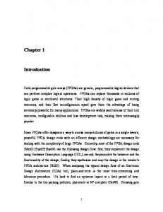
4.11 Three-zone model for microchannel slug flow The three-zone model developed by Thome et al. (2004) describes the evaporation of elongated bubbles in microchannels as a sequential and cyclical passage of a liquid slug (without any entrained vapor bubbles), an evaporating elongated bubble (the film surrounding the bubble is formed from liquid layed down by the liquid slug), and a vapor slug if the liquid film dries out. Figure 17 presents a schematic diagram of this triplet, which repeats over time at the frequency of the bubbles.

Figure 17. Three-zone heat transfer model for elongated bubble flow: a triplet of a liquid slug, an elongated bubble and a vapor slug; flow is from left to right (figure extracted from Thome et al., 2004).

If there is no dry-out, then only a pair of the liquid slug and bubble comprise the model. The local time-averaged heat transfer coefficient at a fixed location z along a microchannel during flow and evaporation of an elongated bubble at a constant, uniform heat flux boundary condition is modeled as: ℎ 𝑧 =

!! !

ℎ! 𝑧 +

!!"#$ !

ℎ!"#$ 𝑧 +

!! !

ℎ! 𝑧

(54)

where τ is a period of pair generation in the original formulation of this model in Jacobi and Thome (2002) assuming it was the time for a spherical bubble to grow across the channel diameter: 𝑓=

! !

=

!! !!,! !!!"# ! !"!!,! !! !!!" !

!

(55)

26


and Dt,l is the thermal diffusivity of the liquid in m2s-1. A new expression of frequency was derived from the database and is presented later. The following assumptions have been made to develop the three-zone model: • The two-phase flow is homogeneous, so that the liquid and vapor velocities are equal. • A time-constant heat flux is uniformly distributed over the inner wall of the microchannel. • The temperatures of the liquid and vapor remain at the saturation temperature Tsat, which means that all the energy delivered to the fluid is used for vaporization. • The local saturation temperature is determined based on the vapor pressure curve. • At x = 0 until it grows to the size of the channel diameter, the liquid slug initially contains all liquid that flows past the nucleating bubble. • There is no vapor shear stress on the liquid film, so that the liquid film remains attached to the channel wall as a stagnant liquid. • The film thickness, δ0, is much smaller than the tube radius of R. • The thermal inertia of the channel wall is neglected. The model is initialized with the total mass flow rate given as: !

!!

!

!

𝛤!"!#$ = 𝛤!,! + 𝜋𝑅 !

(56)

and thus the total mass flux is: !

!!

!

!

𝐺!"!#$ = 𝐺 + 𝑅

≈𝐺

(57)

The assumption that Gtotal is equal G is fairly good except for CO2. Furthermore, the initial lengths are for: • a liquid slug 𝐿!,! =

!

𝜏

(58)

𝐿!,! = R

(59)

!!

• vapor ! !

• a pair 𝐿!,! = 𝐿!,! + 𝐿!,! =

! !!

!

𝜏+ 𝑅 !

(60)


27

The length of the tube Lx=1, at which the fluid is totally evaporated is calculated based on the energy balance on the internal surface of the tube with a constant and uniform heat flux boundary condition: 𝛤!"!#$ 1 − 𝑥! Δℎ!" = 𝜋𝑅 ! 𝐺!"!#$ 1 − 𝑥! Δℎ!" = 2𝜋𝑞𝑅𝐿!!!

(61)

where x0 is a mean initial vapor quality, calculated from the mass flow rate of liquid and vapor during one time period of τ: 𝑥! =

!!,!

=

!!,! !!!,!

! !!

!!" !!! !

(62)

Then, substituting Eq. (62) into Eq. (61): 𝐿!!! =

!!!!" !!

𝐺

(63)

Based on the second assumption of the three-zone model, the vapor quality profile along the tube is linear: !!!!

𝑥 𝑧 =

𝑧 + 𝑥!

!!!!

(64)

where z is the axial distance from the point of bubble nucleation at x0. Assuming that the flow is homogeneous, the liquid and vapor velocities are, respectively: 𝑈! =

!!"!#$

!!!

!!

!!!!

𝑈! =

!!"!#$

!

!!

!!

(65) (66)

where εh is the homogeneous cross-sectional void fraction expressed as a function of vapor quality (see Chapter 4): 𝜀! =

! !!

(67)

!!! !! ! !!

since the volumetric void fraction for this special case is identical to the crosssectional void fraction. Finally, the velocity of the pair is: 𝑈! = 𝐺!"!#$

! !!

+

!!! !!

(68)

Typically, the liquid density ρl is much bigger that the vapor density ρv, so that: 𝑈! ≈ 𝐺!"!#$

! !!

(69)

and the pair/triplet velocity varies nearly linearly along the tube. Following Eq. (68), the mean equivalent length of the pair at each location during one period τ is:

28

J.R. Thome & A. Cioncolini !

𝐿! = 𝜏𝑈! = 𝜏𝐺!"!#$

!!

+

!!!

(70)

!!

and 𝐿! = 1 − 𝜀 𝐿! = 𝜏

!!"!#$

𝐿! = 𝜀𝐿! = 𝜏

!!"!#$

1−𝑥

!! !!

(71)

𝑥

(72)

Then, the time periods that correspond to the presence of a liquid and vapor slugs passing through the cross-section at location z are, respectively: 𝑡! = 𝑡! =

!! !! !! !!

= =

!

(73)

! ! !! ! !! !!!

! ! !!! !! !

(74)

!! !

The model involves the prediction of the initial film thickness, which is difficult to measure experimentally. Starting from the Moriyama and Inoue (1996) correlation, it is described in terms of the Bond number as follows: !!

! ! ∗!.!" !!

!

! ∗!.!"

=

= 0.1 𝑓𝑜𝑟 Bo > 2

0.07𝐵𝑜 !.!"

(75)

𝑓𝑜𝑟 Bo ≤ 2

where d is the tube diameter and Bo is the Bond number as function of the acceleration of the front of the bubble: 𝐵𝑜 =

!! ! ! ! !

!"

𝑈!"#$%&'($ ≃

!! ! ! !!"#$%&'($ !

!!

(76)

In Eq. (75), δ* is the dimensionless boundary layer thickness in front of the bubble: 𝛿∗ =

! ! !!

(77)

!

where tG is the time need for the bubble to reach a particular radius, here tG = d Up-1. In order to ensure the continuity in estimating the initial liquid film over the whole range of conditions, the method of Churchill and Usagi (1972) is employed: !! !

= 𝛿 ∗!.!" 0.07𝐵𝑜 !.!"

!!

+ 0.1!!

!

!!

(78)

Further improvement of the liquid film thickness measurement was provided by Addlesee and Kew (2002) leading to the following formula:

Forced Convective Boiling !! !

= 𝐶!! 3

29

!.!"

!!

0.07𝐵𝑜 !.!"

!! !

!!

+ 0.1!!

!

!!

(79)

where 𝐵𝑜 =

!! ! !

𝑈!!

(80)

The initial thickness of the liquid film will change due to vaporization by the heat flux, q, at the inner wall of the tube. Therefore, based on the third assumption of the three-zone model: 𝑞 2𝜋𝑅Δ𝑧 = −𝜌! 2𝜋 𝑅 − 𝛿

!" !"

Δ𝑧Δℎ!"

(81)

which leads to: 𝑑𝛿 = −

!

!

!! !!!" !!!

𝑑𝑡

(82)

Integrating Eq. (82) with the initial condition 𝛿 𝑧, 0 = 𝛿! 𝑧 and assuming 𝑅 − 𝛿 ≈ 𝑅 gives: 𝛿 𝑧, 𝑡 = 𝛿! 𝑧 −

! !! !!!"

𝑡

(83)

Prior to the heat transfer coefficient calculations, the time periods of film, tfilm, and the dry-out zone, tdry, as well as the final thickness of 𝛿!"# need to be estimated, so that if: • 𝑡!"#,!"#$ > 𝑡! 𝛿!"# 𝑧 = 𝛿 𝑧, 𝑡!

(84)

𝑡!"#$ = 𝑡!

(85)

𝑡!"# = 𝑡! − 𝑡!"#$

(86)

𝐿!"# = 𝑈! 𝑡!"#

(87)

𝛿!"# 𝑧 = 𝛿!"#

(88)

𝑡!"#$ = 𝑡!"#,!"#$

(89)

𝑡!"# = 𝑡! − 𝑡!"#$

(90)

𝐿!"# = 𝑈! 𝑡!"#

(91)

• 𝑡!"#,!"#$ < 𝑡!

where the maximum duration of the existence of the film, tdry,film, at position z is: 𝑡!"#,!"#$ 𝑧 =

!! !!!" !

𝛿! 𝑧 − 𝛿!"#

(92)

30


Now, in Eq. (54), the heat transfer coefficients are: • for liquid film: h 𝑧

!!"#$ !! ! !!"#$ ! ! !,!

𝑑𝑡 =

!! !! !!!"#

!!

𝑙𝑛

(93)

!!"#

• for liquid and vapor slugs: ! ! ℎ! = ℎ!"# + ℎ!"#$

! !

=

! !

! ! 𝑁𝑢!"# + 𝑁𝑢!"#$

! !

(94)

where the average laminar and turbulent Nusselt numbers at z are: !

𝑁𝑢!"#,! = 2×0.455 𝑃𝑟 𝑁𝑢!"#$,! =

! !

!"!!""" !"

!!!".!

! !

!

!"#

(95)

! !

1+

!" ! !!

! ! !

! !

(96)

and 𝜉 = 1.82𝑙𝑜𝑔!" 𝑅𝑒 − 1.64

!!

(97)

The model requires a few constants to be determined based on the experimental results. These are as follows: 1. 𝛿!"# = 0.3, which is the minimum liquid film thickness related to the unknown roughness of the surface and the thermo-physical properties of the fluid, 2. 𝐶!! = 0.29, which is the correction factor on the prediction of 𝛿! taking into account the difference between the fluids and the geometries under investigation, 3. f , which is the pair frequency; its optimum values is estimated as: 𝑓!"# =

!.!"

! !!"#

(98)

and 𝑞!"# = 3328

!!"# !!.! !!"#$

(99)

The values of 𝛿!"# and 𝐶!! , as well as the constants in Eqs. (98) and (99) provided above are applicable in the general three-zone model (Dupont et al., 2004).


31

It has been shown in Costa-Patry et al. (2012) that several modifications to the original heat transfer models of Thome et al. (2004) for elongated bubble flow can be made in order to improve its performance in predicting heat transfer coefficient. Firstly, the model is modified by setting the minimum film thickness to the measured wall roughness since the roughness breaks the liquid film, as shown in Fig. 18. It is worthwhile to mention that this has been already proposed in the previous studies of Agostini et al. (2008) for a multi-microchannel silicon test section, Ong and Thome (2011b) for single stainless steel microtubes, VakiliFarahani et al. (2012) for an aluminum multiport tube, while in the study of Costa-Patry et al. (2012) this was successful for both silicon and copper multimicrochannel test sections.

Figure 18. Three-zone heat transfer model for elongated bubble flow: schematic representation of the transition from film evaporation to vapor convection in the dry zone (figure extracted from Thome et al., 2004).

Secondly, the developing flow Nusselt number correlations were replaced by fully developed ones for laminar and turbulent flow, respectively: 𝑁𝑢!"# = 4.36 𝑁𝑢!"#$ =

! !

(100)

!" !"!!""" !!!".!

! !.! !

!

(101)

!" ! !!

where ξ is a frictional pressure drop coefficient. Then, to stabilize the calculation when the initial and final values of the liquid film were similar, the liquid film heat transfer from Eq. (93) is now given by:

32


ℎ!"#$ =

!! !! !!!"# !!×!"!!

𝑙𝑛

!!

(102)

!!"#

Recently, Magnini et al. (2013a,b) proposed an improvement to the submodel implemented within the three-zone model to better predict the heat transfer in the liquid slug region, according to the results of CFD simulations of slug flow boiling within a microchannel. They observed that the flow within the liquid slug between successive bubbles could be radially split into a recirculating flow occurring at the core of the channel, and a wall adherent layer of liquid which consisted of the liquid that, as dryout did not occur, bypassed the vapor bubble through the thin liquid film region.

Figure 19. Heat transfer coefficient after 21 heated diameters given by the simulation of a slug flow and by the boiling heat transfer model proposed by Magnini et al. (2013a,b).

Using the numerical heat transfer data as the “database”, He et al. (2010) proposed the following correlation:

αS =

k 24.7 + 0.54 Pe0.45 ( LS / d )−1.34 d

[

]

(103)

It computes the average heat transfer coefficient hs at the ideal surface of separation between the wall-adherent and recirculating regions, also called the


33

dividing streamline. Ls is the length of the liquid slug while Pe is the Peclet number of the flow. Figure 19 shows the heat transfer coefficient versus time at a given axial location, processed from the results of a selected slug flow boiling CFD simulation run with the numerical model described in Magnini et al. (2013b). The bypass liquid acts as a thermal resistance to the heat transfer between the recirculating bulk liquid and the channel wall, and is thus responsible for the delay between the end of the liquid film zone and the drop in the heat transfer performance (see the plot within the box in Fig. 19), as opposed to the instantaneous drop predicted by the three-zone model. In order to include the effect of the wall adherent liquid layer into an updated sub-model for the liquid slug zone, the simplified flow configuration depicted in Fig. 20 is considered.

Figure 20. Scheme of the decomposition of the flow field within the microchannel adopted by the two-zone boiling heat transfer model for slug flow of Magnini et al. (2013a,b). R is the radius of the channel.

Note that Figure 20 refers to a two-zone flow decomposition as it was modeled in Magnini et al. (2013b) to emulate the CFD results. Heat is considered to be transferred by one-dimensional transient heat conduction across the adherent liquid layer, such that the following Fourier equation for the heat transfer holds:

∂ 2T ∂T k 2 = ρ cp ∂y ∂t

(104)

where αl identifies the liquid thermal diffusivity. The vertical coordinate y spans from the channel wall (y = 0) to the position of the dividing streamline between wall adherent and recirculating regions (y = δs) within the liquid slug. Equation (104) is solved in time between the end of the liquid film region (t = 0) and the

34


residence time of the liquid slug t = tl. The appropriate boundary conditions are constant wall heat flux q at y = 0, and the following convective condition at y = δ s:

− kl

∂T = hs (T − Ts ) ∂y

(105)

where hs is the heat transfer coefficient at the dividing streamline introduced previously, and Ts is the temperature of the liquid slug. By calculating the heat transfer coefficient as h = k / (Tw - Tsat), with Tw and Tsat being respectively the wall and saturation temperature, the solution of Eq. (104) leads to the following expression for the time-varying heat transfer coefficient at a given axial location during the transit of the liquid slug:

hl (t ) =

1 N

2 1 1 1 + ∑ cme −α l β m tYm (δ s ) + + (Ts − Tsat ) k q m =1 hs q

δs

(106)

where βm and Ym represent respectively the m-th eigenvalue and eigenfunction of the spatial solution of the thermal problem, and cm is a constant which accounts for the initial temperature profile. The denominator of Eq. (106) can be interpreted as the global thermal resistance to the heat transfer between the wall and the bulk liquid within the slug. This includes: (i) the thermal resistance to the heat conduction across the wall adherent liquid layer at the steady state (δs/k) in the 1st term and that during the transient regime (the sum of exponential terms in the 2nd term); (ii) the resistance to the heat convection at the ideal surface of separation between walladherent and recirculating regions (1/ hs) in the 3rd term; and (iii) an equivalent resistance which accounts for the rise in the temperature of the bulk liquid within the slug in the 4th term, which tends to decrease the heat transfer performance as time elapses. In order to implement Eq. (106), closure relationships have to provide values of δs, hs, Ts, tl, and an initial temperature profile. Thulasidas et al. (1997) developed a theoretical model to estimate δs as a function of the bubble velocity. Magnini et al. (2013b) assumed that δs=δ, which was observed to be a valid approximation for δ ≤ D/20. The value of hs is calculated by means of the above correlation proposed by He et al. (2010) and reported in Eq. (103). The timevarying temperature of the liquid slug is given by a simple energy balance between the rear of the bubble at the downstream end of the liquid slug and the axial location under analysis:


35

4qU b t Gc p d

(107)

Ts (t ) = Tsat +

where Ub is the velocity of the bubble, which can be obtained for example by a homogeneous model, G is the mass flux and d is the channel diameter. A method for computing the liquid slug transit time tl is available in Thome et al. (2004) three-zone model described earlier in Eq. (54). The initial temperature profile can be obtained either analytically or as the end temperature profile for the previous zone. The red curve plotted in Fig. 19 displays the heat transfer coefficient obtained by coupling Eq. (106) with a model for the liquid film region presented in Magnini et al. (2013a). This improved model emulates very well the results obtained with the CFD simulation, it is able to capture the trends of the heat transfer in both the transient and the steady-periodic stages and, especially in a later stage the curves overlap. According to Magnini (2013), in order to implement Eq. (106) within Eq. (54) of the three-zone model, the liquid slug heat transfer coefficient has to be integrated in time as follows: t

1 l hl = ∫ hl (t )dt tl 0

(108)

If the sum of exponential terms at the denominator of Eq. (106) can be neglected, Eq. (108) has the following simple analytical solution; otherwise it has to be integrated numerically:

hl =

Gc p d

⎡ 4U t ln⎢1 + b l 4U btl ⎢⎣ Gc p d

⎛ δ s 1 ⎞⎤ ⎜⎜ + ⎟⎟⎥ ⎝ k hs ⎠⎥⎦

(109)

Although this operation can be easily accomplished by implementing any numerical integration method, it is useful to investigate the conditions for which Eq. (109) holds. The sum of exponential terms at the denominator of Eq. (106) drops if the transient stage for the heat conduction across the wall-adherent liquid layer gives a negligible contribution to the average heat transfer coefficient. This condition is verified if the time constant for the heat conduction within the adherent film 1/(αl β12) is much smaller than the transit time of the liquid slug tl. Note that the largest time constant for the thermal transient within the adherent film is associated with the eigenvalue which has the smallest magnitude, i.e. β1. Since β1 is inversely proportional to δs, it follows that the time constant for the transient effect scales as δs2/αl, and hence short thermal transients are promoted by small thicknesses of the wall adherent liquid layer and large values of the

36


liquid thermal diffusivity. For example, Fig. 21 shows some plots of the heat transfer coefficient in the liquid slug zone hl(t) versus time, obtained by means of Eq. (106), for different values of δs2/αl. The working conditions are: fluid R245fa, d = 0.5 mm, G = 550 kgm-2s-1, Tsat = 31 °C, q = 10 kWm-2. The liquid film and liquid slug regions lengths are artificially set respectively to 10d and 30d, and the bubble and liquid slug transit times are evaluated according to an estimated velocity of the bubble of Ub = 0.47 ms-1 which is consistent with the CFD results of Magnini et al. (2013b). The profile of the heat transfer coefficient in the liquid film region (vapor dryout is absent) is obtained by assuming steady state heat conduction across a liquid film of thickness that decreases linearly in time from an initial value of 50 µm to the terminal value of 10 µm. The thickness of the adherent liquid layer is assumed to be 10 µm. The different curves plotted in Fig. 21 are obtained by ranging the liquid thermal diffusivity from 10-10 m2s-1 to 10-6 m2s-1. The thermal transient within the adherent liquid layer becomes negligible for values of δs2/αl on the order of 10-4 s, which is a value that well represents film thicknesses on the order of the micrometer and the thermal diffusivity of many refrigerant fluids (αl ~ 10-8 m2s-1).

Figure 21. Time-dependent heat transfer coefficient in the liquid slug region of a vapor bubble – liquid slug pair obtained by means of Eq. (106): δs2/αl = 10-4, 10-3, 3·10-3, 10-2, 2·10-2, 1 s (from Magnini, 2013).

The value of δs2/αl at which the thermal transient can be considered negligible also depends on the length of the liquid slug, as shorter liquid slugs promote a larger influence of the transient component of the heat conduction across the adherent liquid layer on the average heat transfer coefficient. Figure 22 plots the


37

relative deviation (in % units) of the average heat transfer coefficient obtained by integrating numerically Eq. (106) with (hl) and without (hl,shc, where the subscript shc refers to steady heat conduction) the transient term for heat conduction in the adherent liquid layer, as a function of the liquid slug length, and including the liquid thermal diffusivity as a varying parameter. The liquid thermal diffusivity ranges from 10-8 m2s-1 to 2·10-7 m2s-1, thus well representing refrigerants at typical operating conditions and water at the atmospheric pressure. All the other working conditions are set as reported above, with exception of δs which is set to 5 µm. Figure 22 shows that the use of Eq. (106) without the transient heat conduction term underestimates the average liquid slug heat transfer coefficient by more than 50 % for low thermal diffusivity fluids and liquid slug lengths below 10d. For fluids with a thermal diffusivity above 4·10-8 m2s-1, the transient term can be disregarded for Ls > 20d as the error in the average heat transfer coefficient for the liquid slug drops below 15 %.

Figure 22. Deviation between the average liquid slug heat transfer coefficient given by Eq. (106) with (hl) and without the transient heat conduction term (hshc, shc: steady heat conduction). αl=108 , 2·10-8, 4·10-8, 6·10-8, 8·10-8, 10-7, 2·10-7 m2s-1 (from Magnini, 2013).

4.12 Flow pattern based model for microchannels The three-zone slug flow and the annular flow heat transfer models described above have been combined to make a flow pattern based model for flow boiling in microchannels by Costa-Patry and Thome (2013). In particular, this is done in three steps. First of all, the transition boundary between the two flow patterns is predicted, secondly a transition range around this boundary is assumed where

38


both heat transfer mechanisms are contributing, and thirdly a “mixing” law is assumed to smoothly join the predicted value of the heat transfer coefficient from the three-zone model with that of annular flow model (both for circular and noncircular channels) to mesh their two contributions together. For the first step, an updated transition equation of the prior Revellin and Thome (2007b) and Ong and Thome (2011) transitions was proposed for xCB/A between the slug flow (CB) and the annular flow (A) regimes by Costa-Patry and Thome (2013) based on three new experimental heat transfer databases for: (i) a copper multi-microchannel evaporator tested in Costa-Patry and Thome (2013), (ii) a silicon multi-microchannel evaporator tested by Costa-Patry et al. (2011b), and (iii) the extensive test results for three circular tubes (d = 1.03mm, 2.20mm and 3.04mm) presented in Ong and Thome (2011). These results were used to determine the minimum in the measured heat transfer coefficients, which was assumed as the transition vapor quality in these data sets (not actual visualizations). Together these results form a vapor quality transition database covering diabatic conditions with wall heat fluxes from 8 to 260 kWm-2, mass fluxes from 100 to 1100 kgm-2s-1, four different refrigerants (R134a, R1234ze(E), R236fa and R245fa) and diameters from about 0.15 to 3.04 mm. Based on these studies, the vapor quality thresholds were found to be well predicted by the following expression giving the value of xCB/A in in terms of vapor quality (between 0 to 1.0): 0.1

⎛ ρ ⎞ Bo1.1 xCB / A = 425⎜⎜ g ⎟⎟ 0.5 ⎝ ρl ⎠ Co

(110)

Here Bo in this case is the Boiling number (not the Bond number) and Co is the Confinement number, which are defined as follows:

Bo=

q G igl

⎛ ⎞ σ ⎟ Co = ⎜ ⎜ g (ρ − ρ )d 2 ⎟ l g ⎝ ⎠

(111) 1/ 2

(112)

Here, d is the diameter of the circular channel or the hydraulic diameter of a non-circular channel (not the equivalent diameter, which is a circular channel with the same cross-sectional area as the non-circular cross-section and used in the heat transfer expressions). For the second step, a vapor quality transition range xtr is applied to both sides of the transition value xCB/A is determined for “blending region” of the two heat transfer coefficients. To make this work for all


39

test conditions and for those that might be confronted in an application, this is done using the following “flexible” expression:

xtr = xCB / A ± (xexit 5)

(113)

That is, the width of this zone is scaled to be 1/5 of the vapor quality at the exit of the channel or micro-evaporator, xexit. To implement the third step, a proration parameter r is calculated as follows:

r=

x − xCB / A + 0.5 0.4 xexit

(114)

Then, for a linear mixing law (this was written incorrectly in the original paper of Costa-Patry and Thome (2013) whilst applied correctly in their calculations), the following expression was used, evaluated at each local value of x in the range:

h = (1 − r )h3 z + rhA

(115)

Here h3z is that from the three-zone model from its the most recent version of Costa-Patry et al. (2012) who made several modifications to the original heat transfer models of Thome et al. (2004) while hA is from the annular flow model of Cioncolini and Thome (2011) for circular channels, or its modified version for non-circular channels as per Costa-Patry et al. (2011a,b; 2012). These are both discussed in more detail later in Chapter 9. Lamaison (2014) has proposed an improved weighted mixing law that better represents the shallow minima found in the heat transfer data sets noted above and this is given as:

h=

(1 − r )h32z + rhA2 (1 − r )h3 z + rhA

(116)

With this new weighted mixing law, the heat transfer coefficient data sets for several 0.1 mm square multi-microchannel evaporators extensively tested for R236fa and R245fa by Szczukiewicz et al. (2013) were better predicted compared to the linear law, where it was already shown in that study that the prediction method of Costa-Patry and Thome (2013) for the transition value xCB/A worked well without modification for predicting the location of the minimum. Figure 23 illustrates the incorrect linear mixing law, the correct linear mixing law and the new weighted mixing law applied to the transition range of r from 0 to 1.0.

40


Figure 23. Example of mixing law calculations (points) for microchannel flow pattern-based flow boiling model.

5. Nomenclature Bo Bo cp d Dtl e f g G h h3z hA Δhlv, igl

Bond number (-) Boiling number (-) fluid specific heat (Jkg-1K-1) tube diameter (m) liquid thermal diffusivity (m2s-1) entrained liquid fraction (-) frequency (Hz) acceleration of gravity (ms-2) mass flux (kgm-2s-1) heat transfer coefficient (Wm-2K-1) three-zone model heat transfer coefficient (Wm-2K-1) annular flow model heat transfer coefficient (Wm-2K-1) fluid latent heat (Jkg-1)


k L Nu q, qwall Pr r R Re Tsat Twall U x xCB/A xexit xtr z Γ µg µl ε εh ρg, ρv ρl σ τ

41

thermal conductivity (Wm-1K-1) length (m) Nusselt number heat flux (Wm-2) Prandtl number proration parameter (-) tube radius (m) Reynolds number fluid saturation temperature (K) heated channel wall temperature exposed to the flow (K) velocity (ms-1) vapor quality (-) coalescing bubble to annular flow transition vapor quality (-) channel or evaporator exit vapor quality (-) left or right transition boundary vapor quality (-) axial coordinate along heated channel (m) mass flow rate (kgs-1) gas viscosity (kgm-1s-1) liquid viscosity (kgm-1s-1) cross sectional void fraction (-) homogeneous void fraction (-) vapor density (kgm-3) liquid density (kgm-3) surface tension (kgs-2) period of liquid slug-bubble pair generation (s)

Subscripts: fc film g, v go l lo la lam pb turb

forced convective liquid film vapor only vapor only liquid liquid only liquid all laminar pool boiling turbulent

42


6. References Addlesee, A.J. and Kew, P.A., (2002). Development of the liquid film thickness above a sliding bubble. Trans. Inst. Chem. Eng. 80, pp. 272–277. Agostini, B., Thome, J.R., Fabbri, M., Michel, B., Calmi, D. and Klote, U., (2008). High heat flux flow boiling in silicon multi-microchannels – Part I: Heat transfer characteristics of refrigerant R236fa. Int. J. Heat Mass Transfer 51, pp. 5400–5414. Bertoletti, S., Lombardi, C. and Silvestri, M., (1964). Heat transfer to steam-water mixtures. CISE Report R-78, Segrate, Italy. Bergles, A.E. and Rohsenow, W.M., (1964). The determination of forced convection surface boiling heat transfer. ASME J. Heat Transfer 86, pp. 356-372. Bergles, A.E., Collier, J.C., Delhaye, J.M., Hewitt, G.F. and Mayinger, F., (1981). Two-Phase Flow and Heat Transfer in the Power and Process Industries. McGraw-Hill, New York, USA. Brennen, C.E., (2006). Fundamentals of Multiphase Flow. Cambridge University Press, New York, USA. Bjorge, R.W., Hall, G.R. and Rohsenow, W., (1982). Correlation of forced convection boiling heat transfer data. Int. J. Heat Mass Transfer 25, pp. 753-757. Borishanskij, B.M., Andreevskij, A.A., Fromzel, V.N., Fokin, B.S., Cistgakov, V.A., Danilowa, G.N. and Bikov, G.S., (1971). Heat transfer during two-phase flows (in Russian). Teploenergetika 11, pp. 68-69. Chen, J.C, (1966). Correlation for boiling heat transfer to saturated fluids in convective flow. Ind. Eng. Chem. Proc. Des. 5, pp. 322-329. Churchill, S.W. and Usagi, R., (1972). A general expression for the correlation of rates of transfer and the other phenomena. AIChE J. 18, pp. 1121–1128. Cioncolini, A., Santini, L. and Ricotti, M.E., (2007). Effects of dissolved air on subcooled and saturated flow boiling of water in a small diameter tube at low pressure. Exp. Therm. Fluid Sci. 32, pp. 38-51. Cioncolini, A. and Thome, J.R., (2011). Algebraic turbulence modeling in adiabatic and evaporating annular two-phase flow. Int. J. Heat Fluid Flow 32, pp. 805-817. Cioncolini, A., Thome, J.R. and Lombardi, C., (2009). Unified macro-to-microscale method to predict two-phase frictional pressure drops of annular flows. Int. J. Multiphase Flow 35, pp. 1138-1148. Cioncolini, A. and Thome, J.R., (2012). Entrained liquid fraction prediction in adiabatic and evaporating annular two-phase flow. Nucl. Eng. Des. 243, pp.200-213. Cooper, M.G., (1984). Saturation nucleate pool boiling. A simple correlation. Inst. Chem. Eng. Symp. Ser. 86, pp. 785-793. Costa-Patry, E., Olivier, J., Michel, B. and Thome, J.R., (2011a). Two-phase flow of refrigerants in 85µm-wide multi-microchannels: part I – pressure drop. Int. J. Heat and Fluid Flow 32, pp. 451-463. Costa-Patry, E., Olivier, J., Michel, B. and Thome, J.R., (2011b). Two-phase flow of refrigerants in 85µm-wide multi-microchannels: part II – heat transfer with 35 local heaters. Int. J. Heat and Fluid Flow 32, pp. 464-476. Costa-Patry, E., Olivier, J. and Thome, J.R., (2012). Heat transfer characteristics in a copper microevaporator and flow pattern-based prediction method for flow boiling in microchannels, Frontiers in Heat and Mass Transfer 3, www.ThermalFluidsCentral.org, paper 013002.


43

Costa-Patry, E., Thome, J.R., (2013). Flow pattern based flow boiling heat transfer model for microchannels. Int. J. Refrigeration 36, pp. 414-420. Dittus, P.W. and Boelter, L.M.K., (1930). Heat transfer in automobile radiators of the tubular type. Univ. Calif. Pub. Eng. 2, pp. 443-461; reprinted in Int. Comm. Heat Mass Transfer (1985) pp. 3-22. Dupont, V., Thome, J.R. and Jacobi, A.M., (2004). Heat transfer model for evaporation in microchannels. Part II: comparison with the database. Int. J. Heat Mass Transfer 47, pp. 3387–3401. Forster, H.K. and Zuber, N., (1955). Dynamics of vapor bubbles and boiling heat transfer. AIChE J. 1, pp. 531-535. Gungor, K.E. and Winterton, R.H.S., (1986). A general correlation for flow boiling in tubes and annuli. Int. J. Heat Mass Transfer 29, pp. 351-358. Gungor, K.E. and Winterton, R.H.S., (1987). Simplified general correlation for saturated flow boiling and comparisons of correlations with data. Chem. Eng. Res. Des. 65, pp. 148-156. He, Q., Hasegawa, Y. and Kasagi, N., (2010). Heat transfer modeling of gas-liquid slug flow without phase change in a micro tube. Int. J. Heat Fluid Flow 31, pp. 126-136. Hewitt, G.F., (1998). Boiling. In: Rohsenow, W.M., Hartnett, J.P., Cho, Y.I. (Eds.), Handbook of Heat Transfer, McGraw Hill, New York. Jacobi, A.M. and Thome, J.R., (2002). Heat transfer model for evaporation of elongated bubble flows in microchannels, ASME J. Heat Transfer 124, pp. 1131-1136. Kandlikar, S.G., (1990). A general correlation for saturated two-phase flow boiling heat transfer inside horizontal and vertical tubes. ASME J. Heat Transfer 112, pp. 219-228. Kattan, N., Thome, J.R. and Favrat, D., (1998). Flow boiling in horizontal tubes. Part 3: development of a new heat transfer model based on flow patterns. ASME J. Heat Transfer 120, pp. 156-165. Kenning, D.B.R. and Cooper, M.G., (1989). Saturated flow boiling of water in vertical tubes. Int. J. Heat Mass Transfer 32, pp. 445-458. Lamaison, N., (2014). Dynamic Modeling and Experimental Evaluation of a Controlled Two-Phase On-Chip Cooling System designed for High Efficiency Datacenter, PhD thesis, Ecole Polytechnique Fédérale de Lausanne. Liu, Z. and Winterton, R.H.S., (1991). A general correlation for saturated and subcooled flow boiling in tubes and annuli, based on a nucleate pool boiling equation. Int. J. Heat Mass Transfer 34, pp. 2759-2766. Lockhart, R.W. and Martinelli, R.C., (1949). Proposed correlation of data for isothermal two-phase, two-component flow in pipes. Chem. Eng. Progr. 45, pp. 39-48. Magnini, M., (2013). Personal communication. Magnini, M., Pulvirenti, B. and Thome, J.R., (2013a). Numerical investigation of hydrodynamics and heat transfer of elongated bubbles during flow boiling in a microchannel. Int. J. Heat Mass Transfer 59, pp. 451-471. Magnini, M., Pulvirenti, B. and Thome, J.R., (2013b). Numerical investigation of the influence of leading and sequential bubbles on slug flow boiling within a microchannel. Int. J. Thermal Sci. 71, pp. 36-52. Mikic, B.B. and Rohsenow, W.M., (1969). A new correlation of pool boiling data including the effect of heating surface characteristics. ASME J. Heat Transfer 91, pp. 245-251. Moriyama, K. and Inoue, A., (1996). Thickness of the liquid film formed by a growing bubble in a narrow gap between two horizontal plates. ASME J. Heat Transfer 118, pp. 132–139.

44


Ong. C.L. and Thome, J.R., (2009). Flow boiling heat transfer of R134a, R236fa and R245fa in a horizontal 1.030 mm circular channel. Exp. Therm. Fluid Sci. 33, pp. 651-663. Ong. C.L. and Thome, J.R., (2011). Macro-to-microchannel transition in two-phase flow: part 2flow boiling heat transfer and critical heat flux. Exp. Therm. Fluid Sci. 35, pp. 873-884. Revellin, R. and Thome, J.R., (2007). A new type of diabatic flow pattern map for boiling heat transfer in microchannels. J. Micromechanics and Microengineering 17, pp. 788-796. Rouhani, S.Z. and Axelsson, E., (1970). Calculation of void volume fraction in the subcooled and quality boiling regions. Int. J. Heat Mass Transfer 13, pp. 383-393. Saitoh, S., Daiguji, H. and Hihara, E., (2007). Correlation for boiling heat transfer of R134a in horizontal tubes including effect of tube diameter. Int. J. Heat Mass Transfer 50, pp. 52155225. Szczukiewicz, S., Borhani, N. and Thome, J. R., (2013). Fine-resolution two phase flow heat transfer coefficient measurements of refrigerants in multi-microchannel evaporators. Int. J. Heat Mass Transfer 67, pp. 913-929. Shah, M.M., (1976). A new correlation for heat transfer during boiling flow through pipes. ASHRAE Trans. 82, pp. 66-86. Shah, M.M., (1982). Chart correlation for saturated boiling heat transfer: equations and further study. ASHRAE Trans. 88, pp. 185-196. Shin, J.Y., Kim, M.S. and Ro, S.T., (1997). Experimental study on forced convective boiling heat transfer of pure refrigerants and refrigerant mixtures in a horizontal tube. Int. J. Refrig. 20, pp. 267-275. Silvestri, M., Casagrande, I., Cravarolo, L., Hassid, A., Bertoletti, S., Lombardi, C., Peterlongo, G., Soldaini, G., Vella, G., Perona, G. and Sesini, R., (1963). A Research Program in Two-Phase Flow. CISE Report, Segrate, Italy. Steiner, D., (1987). Evaporation in horizontal tubes. In: Hewitt, G.F., Delhaye, J.M., Zuber, N. (Eds), Multiphase Science and Technology, Vol. 3, Hemisphere, Washington. Stephan, K. and Abdelsalam, M., (1980). Heat transfer correlation for natural convection boiling. Int. J. Heat Mass Transfer 23, pp. 73-87. Thome, J.R., Dupont, V. and Jacobi, A.M., (2004). Heat transfer model for evaporation in microchannels. Part I: presentation of the model. Int. J. Heat Mass Transfer 47, pp. 3387– 3401. Thulasidas, T.C., Abraham, M.A. and Cerro, R.L., (1997). Flow patterns in liquid slugs during bubble-train flow inside capillaries. Chem. Eng. Sci. 52, pp. 2947-2962. Tibiriçá, C.B. and Ribatski, G., (2010). Flow boiling heat transfer of R134a and R245fa in a 2.3 mm tube. Int. J. Heat Mass Transfer 53, pp. 2459-2468. Vakili-Farahani, F., Agostini, B. and Thome, J.R., (2012). Experimental study on flow boiling heat transfer of multiport tubes with R245fa and R1234ze(E), ECI 8th International Conference on Boiling and Condensation Heat Transfer, Lausanne, Switzerland, 3-7 June. Zhang, W., Hibiki, T. and Mishima, K., (2004). Correlation for flow boiling heat transfer in minichannels. Int. J. Heat Mass Transfer 473, pp. 5749-5763.

Chapter 7 Forced Convective Boiling 1. Introduction

Chapter 7 Forced Convective Boiling 1. Introduction

Suggest Documents

Forced Convective Boiling of Hydrocarbon Mixtures

Forced Convective Boiling of Hydrocarbon Mixtures - MAFIADOC.COM

Forced convective boiling in vertical tube for binary ... - Springer Link

Bubble departure frequency in forced convective subcooled boiling flow

experimental study on forced convective boiling of ... - CiteSeerX

experimental study on forced convective boiling of ... - CiteSeerX

ChAPTEr 7 Introduction - OFAC

Chapter 1 Introduction Chapter 1

CHAPTER 7 - EARTHWORKS 7.0 INTRODUCTION This chapter ...

Chapter 1 INTRODUCTION 1

chapter-1 1. introduction

Chapter 7 Introduction to Sampling

modelling convective boiling of molasses - CSIRO CFD

Download Convective Boiling and Condensation ... - Google Sites

CHAPTER 1 INTRODUCTION 1.1 Introduction

Chapter 7 Chapter 7

chapter 1: introduction

Chapter 1: Introduction

Chapter 1 Introduction

chapter 1 introduction

Chapter 1: Introduction - arXiv

chapter 1: introduction

Chapter 1 Introduction

Chapter 1: Introduction - Wiley