deep neural network methods, many models have been pro- posed to ... text representations may not represent word meanings well ..... segmentation, named entity recognition for Chinese), and ... larity score by twelve native speakers according to their sim- .... the intended meaning of a word in context independently of ...
Learning Context-Specific Word/Character Embeddings Xiaoqing Zheng, Jiangtao Feng, Yi Chen, Haoyuan Peng, Wenqing Zhang School of Computer Science, Fudan University, Shanghai, China Shanghai Key Laboratory of Intelligent Information Processing {zhengxq, fengjt16, yi chen15, hypeng15, wqzhang}@fudan.edu.cn
Abstract Unsupervised word representations have demonstrated improvements in predictive generalization on various NLP tasks. Most of the existing models are in fact good at capturing the relatedness among words rather than their “genuine” similarity because the context representations are often represented by a sum (or an average) of the neighbor’s embeddings, which simplifies the computation but ignores an important fact that the meaning of a word is determined by its context, reflecting not only the surrounding words but also the rules used to combine them (i.e. compositionality). On the other hand, much effort has been devoted to learning a singleprototype representation per word, which is problematic because many words are polysemous, and a single-prototype model is incapable of capturing phenomena of homonymy and polysemy. We present a neural network architecture to jointly learn word embeddings and context representations from large data sets. The explicitly produced context representations are further used to learn context-specific and multiprototype word embeddings. Our embeddings were evaluated on several NLP tasks, and the experimental results demonstrated the proposed model outperformed other competitors and is applicable to intrinsically “character-based” languages.
Introduction and Motivation Much recent research has been devoted to deep learning algorithms which achieved impressive results on various natural language processing (NLP) tasks. The best results obtained on supervised learning tasks involve an unsupervised learning phase, usually in an unsupervised pre-training step to learn distributed word representations (also known as word embeddings). Such semi-supervised learning strategy has been empirically proven to be successful by using unlabeled data to supplement the supervised models for better generalization (Collobert et al. 2011; Socher et al. 2011; dos Santos and Zadrozny 2014; Zheng, Chen, and Xu 2013; Pei, Ge, and Chang 2014). Due to the importance of unsupervised pre-training in deep neural network methods, many models have been proposed to learn word embeddings. The two main model families are: (a) predicting or scoring the target word based on its local context, such as the neural probabilistic language c 2017, Association for the Advancement of Artificial Copyright Intelligence (www.aaai.org). All rights reserved.
model (NNLM) (Bengio et al. 2003), C&W (Collobert et al. 2011), and continuous bag-of-words (CBOW) (Mikolov et al. 2013a); (b) using a word to predict its surrounding words, such as the Skip-gram (Mikolov et al. 2013a) as well as its extensions, multi-sense Skip-gram (MSSG) (Neelakantan et al. 2014) and proximity-ambiguity sensitive (PAS) Skipgram (Qiu et al. 2014). However, they suffer one or both of the following significant drawbacks. First, the context is often represented by a sum (or an average) of the surrounding words’ feature vectors. Those context representations may not represent word meanings well because the meaning of a word is affected by its adjacent words and the rules to combine them. Each context word in general does not contribute equally to the meaning of the target word, and thus the simple sum or average operation can not capture this compositionality. Second, most of the existing methods create a singleprototype embedding for each word. This single-prototype representation is problematic because many words are intrinsically polysemous, and a single-prototype model is incapable of capturing phenomena of homonymy and polysemy. It is also important to be reminded that languages differ in the degree of polysemy they exhibit. For example, Chinese with its (almost) complete lack of morphological marking for parts of speech certainly exhibits a higher degree of polysemy than English (Packard 2004). Recent models on learning multiple representations per word (Reisinger and Mooney 2010; Huang et al. 2012) generally work as follows: for each word, first cluster its contexts into a set of clusters, and then derive multiple representations (each for a cluster) of the word from the clusters of similar contexts. In these models, each context is represented by a vector composed of the occurrences of its neighboring words or a weighted average of the surrounding words’ vector. Such context definitions neglect the relative order of words in the context window, which impairs the quality of the multi-prototype representations derived by the clustering based on such context representations. In fact, the order of words does matter to the meaning of those they form. Besides, those models set the equal number of prototypes for each word, although different numbers were tested to determine the optimal number of prototypes. We argue that the degree of polysemy in polysemous words depends on the number of distinct contexts in which
Context-Specific Vector Model Many methods were proposed to learn distributed word representations from large unlabeled texts, but the questions still remain as to how meaning is produced by such unsupervised methods, and how the resulting word vectors represent that meaning. We describe here a neural networkbased model, named CSV (Context-Specific Vector), which can generate the context representation of a word/character, and learn the word/character vector carrying the meaning inferred by that context. The proposed network architecture contains a convolutional layer that is designed to produce the refined context representations reflecting the order of their constituents and the rules to combine them. The better generated context representations are used to learn contextspecific multi-prototype word/character embeddings by the sense induction with a simple “winner-takes-all” strategy.
consider a fixed-sized type dictionary D. The type’s global vectors are stored in a matrix M ∈ Rd×|D| , where d is the dimensionality of the vector space (a hyper-parameter to be chosen) and |D| is the size of the dictionary. Word/Character Context g(t−w/2) • • • g(t−1) g(t+1) • • • g(t+w/2) 1 2 3 .. . d−1 d
Lookup Table Global Vectors
Window Size Convolution
Context Representation
s1(t0)
Sense prediction by win-takes-all strategy
s2(t0)
sk(t0) .. .
they occur, especially for the “character-based” languages (e.g. Chinese and Japanese). When a word appears in more different linguistic contexts, it may carry more meanings, and greater number of prototypes should be created for that word. It is unnecessary for rare words to learn several prototypes, whereas for most common words, if the number of word senses is greater than that of prototypes, certain prototype could be affected by the contexts associated with different meanings, and the learned prototype might not represent any one of the meanings well as it is influenced by several (and different) meanings of that word. We present a novel neural network architecture to learn multi-prototype word/character embeddings from large data sets, in which the context representations are produced by a convolutional layer, designed to capture the compositionality of context words or characters. This architecture allows us to take advantage of the better trained context representations and to learn multi-prototype word/character embeddings accordingly. The number of prototypes for each word/character can be different and selected automatically. Experimental results show that the embeddings learned by our model outperform competitors on the several NLP tasks across different languages by transferring the unsupervised representations into the supervised models.
Word/Character Sense Vectors
Figure 1: The neural network architecture. The context feature window produced by the first lookup table is a matrix H ∈ Rd×w , where each column of the matrix H is the global vector of the type in the window. A onedimensional convolution is used to yield another feature vector by taking the dot product of filter vectors with the rows of the matrix H at the same dimension. After each row of H is convolved with the corresponding column of a filter matrix W, the context features are extracted as follows. F =H W
(1) w×d
where the weights in the matrix W ∈ R are the parameters to be trained, and F ∈ Rd is a vector. The trained weights in W can be viewed as a linguistic feature detector that learns to recognize a specific class of n-gram (Kalchbrenner, Grefenstette, and Blunsom 2014). The context feature vectors from a window of text can be computed efficiently thanks to one-dimensional convolution.
Training The Neural Network Architecture The network architecture is shown in Figure 1. From now on, a term “type” is used to refer to word or character, depending on which language is considered (e.g. word in English or character in Chinese). Each type is associated with a global vector and multiple sense vectors. The input to the network is a type’s context window, and the convolutional layer produces the representation (or vector) for that context. One of the type’s sense vectors is chosen by how well the sense fits into the context, and the network is trained to differentiate the selected sense vector from others. We use a window approach that assumes the meaning of a type depends mainly on its surrounding types. The types (except the target) in the window of size w (a hyper parameter) are fed into the network as indices that are used by a lookup operation to transform types into their global vectors. We
We start with the description of learning in single-prototype case (i.e. each type has a unique sense vector), and then extend it to multi-prototype situation. Once the context representation is generated, we use that representation to discriminate the target type from the others. Like (Mikolov et al. 2013b), a negative sampling method is applied to approximately maximize the probability of the target type given its context. The neural networks are trained by maximizing the conditional likelihood of the target types given their contexts using the gradient ascent algorithm. The log-likelihood function we consider takes the following form: XX l(θ) = log pθ (t|c) (2) t∈D c∈Ct
where D is the dictionary of types, Ct is the set of all possible context windows the type t occurs (the target type is
removed), and θ are the parameters needed to be trained. The distribution pθ (t|c) can be factorized with respect to the type t itself (positive) and its negative samples using logistic regression as follows. Q pθ (t|c) = pθ (x|c) x∈{t}∪neg(t) � (3) φ(s(x)> v(c)), if x = t; pθ (x|c) = > 1 − φ(s(x) v(c)), if x ∈ neg(t).
online during training when the type is observed with a context that the cosine similarity between the context feature vector with every existing sense vector is less than a threshold δ (a hyper-parameter). Ideally, the context vectors should be generated by using the sense vectors. We choose to use the global vectors of the context types instead of their sense vectors to avoid the high computational cost caused by the sense disambiguation for the context types.
where v(c) is t’s context vector representation produced by the convolutional layer, s(·) is the type’s sense vector, neg(t) is a set of negative samples drawn for each occurrence of the type t, and φ(·) is a sigmoidal function. These lead us to maximize the following objective function: P P l(θ) = {log[φ(s(t)> v(c))]+ t∈D c∈Ct P (4) log[1 − φ(s(x)> v(c))]}
Inputs: R: a training corpus. K: a specified number of negative samples. N : a specified number of iterations. Initialization: the parameters of the network, a global vector g(t) and a sense vector s(t) for each type t ∈ D are initialized with small random values. Output: the trained network parameters θ, a global vector g(t) and one or more sense vectors si (t) for each type t ∈ D, i = 1, 2, ..., kt . Algorithm: for STAGE = 1 to 3 do for each context window c in the corpus R. compute the context feature vector v(c) by the neural network using the equation (1). rct = argmaxi sim(si (t), v(c)) for the target type t as the equation (5). if (STAGE = 1 or STAGE = 3) draw a set of K negative samples neg(t) randomly for the target type t. update the network parameters θ, the global vectors of types in the context window, and the rct sense vector of the type t by the gradients with respect to the objective function (4). else if (STAGE = 2) if (sim(srct (t), v(c)) < δ) create a new sense vector for the type t, which is initialized by the context vector v(c). else update the sense vector srct (t) to reflect the influence of the current context feature vector v(c). until the number of iterations N is reached (N = 1 if STAGE 2). end for
x∈neg(t)
When maximizing this log-likelihood, the error will backpropagate and update both the network parameters and type’s vectors.
Multi-Prototype CSV Model In order to learn multiple prototypes, each type could be associated with more than one sense vector. We need to choose a sense vector that most fits into the current context. The “winner-takes-all” principle is used to make this choice, and the sense vector with the highest similarity to the context representation vector is selected to be updated according to the equation (3). More formally, rct = argmax sim(si (t), v(c))
(5)
i=1,2,...,kt
where c ∈ Ct , and the type t has kt sense vectors {s1 (t), s2 (t), ..., skt (t)}. The selected rct is the sense of type t when observed in the context c. For the sim function, we use cosine similarity as a measure of similarity between two vectors. The last question is how many prototypes (or sense vectors) need to be created for each type. We are aware that languages differ in the degree of polysemy they exhibit. For example, Chinese exhibits a higher degree of polysemy than English (Packard 2004). On the other hand, it is necessary to individually determine how many prototypes need to be created for each type. We assume that the degree of polysemy in polysemous types depends on the number of distinct contexts in which they occur, where the context is defined as the combination of neighboring words in a given window. When a type appears in more different linguistic contexts, it may carry more meanings, and greater number of prototypes should be created for that type. For a given corpus, the appropriate number of prototypes for a type is strongly related to the quantity of different contexts in which it occurs, and thus that number should be determined accordingly. Because the appropriate number of sense vectors (to be created) for a type can not be well decided in advance, we try to learn that number during the training in a dynamic way. A new sense vector will be added
Figure 2: The training algorithm of CSV model. The training process is divided into three stages. At first, we expect to learn robust context vector representations. A global vector and a sense vector will be created with random initialization for each type, and the network is in fact trained by single-prototype CSV model. Then, the new sense vectors can be added gradually when necessary. If the cosine similarity between the current context vector and the type’s every existing sense vector is less than a given δ, a new sense vector will be created and initialized with the context vector; otherwise, the sense vector with the highest similarity will be updated with the centroid of the seen context vectors belonging to this sense vector, like the spherical k-mean algorithm. This procedure is closely related to the EM (Expectation-Maximization) algorithm. The E-step of the EM algorithm assigns “responsibilities” for each context vector based in its relative similarity to sense vectors, while
0.8
0.8 CSV-S CBOW SKIP GloVe
CSV-S CBOW SKIP GloVe
0.7
0.7
Spearman's ρ
Spearman's ρ
the M-step recomputes the selected sense vector representation based on the current responsibilities. Finally, the number of sense vectors is fixed for every type, and the new sense vectors are not allowed to be created. At the final stage, we focus on training the context-specific multi-sense vectors. The whole training algorithm is shown in Figure 2.
0.6
0.5
0.5
Experiments
English and Chinese Wikipedia documents1 were used as the unlabeled corpora by all the models compared to train the embeddings because of their wide range of topics and usages. We compared the performance of ours against three state-of-the-art models: GloVe (Pennington, Socher, and Manning 2014), CBOW and SKIP (Mikolov et al. 2013a). All the results reported have been averaged over five runs. For English, a popular data set for evaluating vector-space models is the WordSim-353 (Finkelstein et al. 2001), which has 353 pairs of nouns. Each pair is presented without context and associated with 13 to 16 human judgments on similarity and relatedness by a scale from 0 to 10. Observing that the scores shown in the WordSim-353 data set do not reflect the “genuine” similarity2 , Hill et al (2014) presented the SimLex-999 that explicitly quantifies similarity rather than relatedness or association so that pairs that are related but not actually similar are rated with low scores. For Chinese character similarity task, to the best of our knowledge, there is no such data set available. Following the guidance of (Hill, reichart, and Korhonen 2014), we constructed a CharSim-200 data set, which contains two hundred Chinese character pairs. Each pair is assigned the similarity score by twelve native speakers according to their similarity, and the average of those human judgements was taken as the final score. The scores range from 0 to 10, and the higher the score, the more similar the two characters will be. An average Spearman’s rank correlation coefficient (or 1
https://www.wikipedia.org/ (March 2015 snapshot) In the WordSim-353, “coffee” and “cup” are rated as more similar than pairs such as “car” and “train”. Although the former are very much related, the relationship between those two words is considered as association in the psychological literature, which contrasts with similarity, the relation connecting “cup” and “mug”. 2
3
5
Window Size: 11 7
9
0.4 100
11
200
(a) Window Size
300
400
500
(b) Dimension
Figure 3: Spearman’s ρ on the WordSim-353. (a) Average Spearman’s ρ versus window size with dimension fixed to 300. (b) Average Spearman’s ρ versus dimension with window size fixed to 11. Spearman’s ρ) achieved by human annotators is 0.879, and the highest score is 0.922. 0.6
0.6 CSV-S CBOW SKIP GloVe
CSV-S CBOW SKIP GloVe
0.5
0.5
Spearman's ρ
Comparing with Single-prototype Models
Dimension: 300 0.4
Spearman's ρ
We conducted three sets of experiments. The goal of the first one is to test several variants of the single-prototype CSV model to gain some understanding of how the choices of hyper-parameters impacts the performance on the word and character similarity tasks, by comparing with the wellestablished single-prototype embedding learning methods. In the second experiment, we compare our multi-sense variant with state-of-the-art multi-prototype word representation models on a data set where each word pair is presented with context. The third one is to see how well the learned embeddings to enhance the supervised learning on four standard NLP tasks (POS tagging, chunking for English, and word segmentation, named entity recognition for Chinese), and whether the performance can be further improved by their multi-prototype variants.
0.6
0.4
0.4
0.3
0.3
Dimension: 300
Window Size: 11
0.2 3
5
7
(a) Window Size
9
11
0.2 100
200
300
400
500
(b) Dimension
Figure 4: Spearman’s ρ on the SimLex-999. (a) Average Spearman’s ρ versus window size with dimension fixed to 300. (b) Average Spearman’s ρ versus dimension with window size fixed to 11. We report in Figure 3, 4, and 5 the Spearman’s ρ versus window size and versus vector size for our model and other competitors on the WordSim-353, SimLex999, and CharSim-200 data sets respectively. The proposed singleprototype context-specific vector model is denoted as CSVS. It can be seen from the figures that generally, the larger the dimension, the higher the Spearman’s ρ we will have. We also observed diminishing returns for type vectors with their dimension larger than about 300 both for the WordSim-353 and CharSim-200. The CSV-S achieved steady high performance across the three data sets, while others gave inconsistent performances on the different data sets. As shown in Figure 3, the CSV-S performs comparatively well to the SKIP that achieved the highest Spearman’s ρ of 0.713 (just 0.03 difference to the CSV-S) when the window size was set to 11 and the dimension to 500. It can be seen from Figure 5 that the CSV-S performs similar to the GloVe, and achieved state-of-the-art Spearman’s ρ of 0.805 on the CharSim-200 when the window size was set to 11 and the dimension to 400. For the SimLex999 data set, the CSV-S outperforms the three competitors with a large margin (see Figure 4), and achieved the highest Spearman’s ρ of 0.481. The SimLex999 explicitly quantifies similarity rather than
0.9
0.9 CSV-S CBOW SKIP GloVe
CSV-S CBOW SKIP GloVe
0.8
Spearman's ρ
Spearman's ρ
0.8
0.7
0.7
0.6
0.6
Dimension: 300
Window Size: 11
0.5 3
5
7
9
11
0.5 100
(a) Window Size
200
300
400
500
(b) Dimension
Figure 5: Spearman’s ρ on the CharSim-200. (a) Average Spearman’s ρ versus window size with dimension fixed to 300. (b) Average Spearman’s ρ versus dimension with window size fixed to 11. relatedness, and it was constructed to provide a gold standard resource for evaluating distributional semantic models. The CSV was designed to capture the complicated, but critical semantic “compositionality” of the context windows by using a convolutional layer to learn the refined context representations. The experimental results on the SimLex-999 show that the CSV captures the similarity well, and the performances of other models suffer from their oversimplified context representations.
Comparing with Multi-prototype Models The only one we could find is the Stanford Contextual Word Similarity (SCWS) data set (Huang et al. 2012) that can be used to evaluate multi-prototype models. The data set consists of 2,003 pairs of words and the contexts in which they occur, which makes it possible to select the most appropriate sense for each ambiguous word by its contextual information. We report in Table 1 the Spearman’s ρ between the embedding similarities and human judgments, where our multiprototype context-specific models (CSV-M) is compared against five recently proposed models. Table 1: Spearman’s ρ performance of the multi-prototype models on the SCWS data set. Model Huang et al (2012) Chen et al (2014) Neelakantan et al (2014) Cheng and Kartsaklis (2015) Iacobacci et al (2015) CSV-M
Spearman’s ρ 0.657 0.689 0.691 0.585 0.624 0.699
The CSV-M achieved the best Spearman’s ρ of 0.699 on the SCWS, which was calculated by the similarity between each pair of sense vectors, selected independently based on their contexts. The values of hyperparameters were chosen by a small amount of manual exploration on a validation set. The network was trained by setting the windows size to 11, the dimension to 300, and δ to 0.15. It is worth noting that the comparison is indirect because many other models often use some external sources or weighted average methods to
improve their performances. For example, the sense vectors of (Chen, Liu, and Sun 2014) were generated with the help of the WordNet (Miller 1995). A state-of-the-art word sense disambiguation tool was applied by Iacobacci et al (2015) to generate the sense-annotated corpora that were used to train multi-sense embeddings. The best performances reported in both (Huang et al. 2012) and (Neelakantan et al. 2014) were all achieved by weighting the similarity between each pair of sense vectors by how well does each sense fit the context. The performance of (Neelakantan et al. 2014) drops to 0.598 if the similarity between two words was computed by selecting a single sense for each word based on its context like the CSV-M did. In comparison, the results were obtained by the CSV-M without using any extra information.
Results on four NLP Tasks This section describes four downstream NLP tasks on which different models are evaluated: POS-tagging, chunking, Chinese word segmentation (CWS) and named entity recognition (NER). For the English POS-tagging, the performance is reported in per-word accuracy. The other three tasks are evaluated by computing the standard F1-score, which is the harmonic mean of precision and recall. We assume that one can take an existing, close to stateof-the-art, supervised NLP system, and its performance can be further improved by transferring the unsupervised embeddings into the system. We implemented the neural network of (Collobert et al. 2011) as such supervised component, which was designed to perform the sequence labeling tasks. The network will output the scores for all the possible labels for the task of interest. The POS-tagging task consists of marking up the syntactic role for each word. For the remaining three tasks, we use the most expressive “IOBES” tagging scheme. • Part-of-speech tagging aims at marking up a word in a sentence with a unique label that indicates its syntactic role, such as noun, verb, adjective, etc. We used a benchmark setup described by Toutanova et al (2003). • Chunking (also known as shallow parsing) is an analysis of a sentence which identifies syntactic constituents such as noun or verb phrases. Chunking is often evaluated using the CoNLL 2000 shared task. • Word segmentation is to reconstruct the word boundaries of texts in those languages that are written without using whitespace to delimit words. We picked Penn Chinese Treebank from Bakeoff-3 as our data set (Levow 2006). • Named entity recognition seeks to locate and classify elements in the sentence into pre-defined categories such as the names of persons, organizations, locations, etc. For the NER task, we choose MSRA data set from Bakeoff-3 with standard train-test splits (Levow 2006).
For the CSV-M, each type in the training and testing corpora was relabeled with its corresponding sense, and the combination of type and sense label is considered as one type. Generally, word sense disambiguation is a computationally expensive step because the algorithms have to consider all possible combinations of occurring senses on a sentence (up to k n sense sequences for a sequence of n words when each has up to k sense). However, the CSV-M chooses the intended meaning of a word in context independently of
the sense labels of its surrounding words, and thus the relabeling step runs in linear time. Because there is no direct way to obtain the sense labels from other multi-prototype models, we just compared the existing single-prototype models against ours. For the models to be evaluated here, the dimension was set to 300, and the window size to 11. Table 2: Comparison with the previous embedding learning models. Model Baseline CBOW SKIP GloVe CSV-S CSV-M
POS (PWA) 95.40 95.50 96.06 95.86 96.26 97.15
CHUNK (F1) 89.10 89.37 89.77 89.18 91.49 92.12
CWS (F1) 92.15 92.55 92.83 92.99 93.26 94.03
NER (F1) 82.03 82.53 84.02 82.56 85.31 85.59
The results shown in Table 2 suggest that unsupervised pre-training gives consistently better generalization comparing to the baseline started with randomly initialization (without pre-training embeddings), and the CSV-S boosts the performances of all the tasks by a fairly significant margin, particularly for the chunking (1.72% in average) and NER (1.29% in average). The results also show that its multiprototype enhancements, CSV-M, can further improve the performances. The results for four benchmark data sets show that our models achieved consistently higher performance over the three competitors.
Related Work Over the last decade, there has been increasing interest in learning word representations from a large collection of unlabeled data, and using these word representations as a feature set to augment the supervised learners. Generally, related work on learning word representations can be divided into three categories: clustering-based (Brown et al. 1992; Li and McCallum 2005), distributional (Teh et al. 2006; ˘ u˘rek and Sojka 2010), and distributed representations Reh˚ (Bengio et al. 2003; Collobert and Weston 2008). In this paper, we focus on the distributed representation models. Distributed word representations are also called word embeddings, each dimension of which represents latent feature about word syntactic and semantic information. The goal of (Bengio et al. 2003) is to estimate the probability of a word given the previous words in a sentence using the cross-entropy criterion. Because the size of dictionary is usually large, the computation of exponentiation and normalization can be extremely demanding, and sophisticated approximations are required. Many approaches have been proposed to eliminate the linear dependency on the dictionary size. The model of (Mnih and Hinton 2007) learns a linear model to predict the embedding of the last word given the concatenation of the embeddings of previous words. Collobert and Weston (2008) introduced a neural language model that evaluates the acceptability of a piece of text. The related studies closest to ours in term of handling multi-prototype word representations are (Reisinger and
Mooney 2010; Huang et al. 2012; Qiu et al. 2014; Neelakantan et al. 2014). Reisinger and Mooney (2010) introduced a multi-prototype vector-space model, where multiple prototypes for each word are generated by clustering contexts of the word occurrence and collecting the resulting cluster centroids. The dimensionality of their word vectors is normally large, which corresponds to the size of vocabulary. Huang et al (2012) presented a neural language model that learns the word embeddings by incorporating both local (previous words) and topic (document vectors) information. The single-prototype embeddings learned in advance are used to represent the word context, and these context representations are then clustered by spherical k-means using cosine distance. Multiple prototypes of a word are induced from its associated clusters. For multi-prototype variants, they fix the number of prototypes to be ten. It shows that the performance is sensitive to the number of prototypes, and the number of prototypes created for each word should be determined individually. Qiu et al (2014) addressed the word-sense discrimination problem by creating multiple representations per word, each for a POS type. However, many words may still carry more than one meaning even though they are constrained to a certain POS type. A POS tagger can effectively process the texts from the same domain as the training texts, but the performance may deteriorate significantly when the tagger is used to the large texts from others, which is not conducive to the word-sense discrimination. They used a weighted average of the context word vectors to represent the context. In comparison, we model the refined contexts by a convolutional layer, particularly to capture the their semantic interpretations and compositions of the context words. Neelakantan et al (2014) extended the Skip-gram model to learn multi-prototype word embeddings from large unlabeled texts by adding a word-sense disambiguation layer to the network. The sense disambiguation works by maintaining multiple sense vectors per word and identifying the sense whose vector is the closest to the current context. The word sense vectors are initialized randomly and updated together with the word embeddings during the training. Their model follows the philosophy behind the Skip-gram, using the target word to predicting its context words, while our word embeddings are learned by making them well suited for the co-trained context representations. In addition, the word context is represented as an average of its surrounding word’s vectors in their model, which might not be well enough to represent the meaning (i.e. compositionality) of the context words and would lead to poor clustering results.
Conclusion Word or character embeddings can be learned in advance in an unsupervised manner. These embeddings, once learned, are easily disseminated with other researchers, and easily integrated into existing supervised NLP systems. We presented a novel neural network architecture as well as a context-specific vector model that can learn multi-prototype word/character representations, which are capable of capturing word’s or character’s syntactic and semantic information, particularly their polysemous variants. Our model
differs from recent related work by jointly learning the context representations and embeddings, and by estimating the number of senses per word/character type. Experiment results with different datasets showed that the proposed model outperformed the existing state-of-the-art embedding learning methods on several NLP tasks across two languages.
Acknowledgments The authors would like to thank the anonymous reviewers for their valuable comments. This work was supported by a grant from Shanghai Municipal Natural Science Foundation (No. 15511104303).
References Bengio, Y.; Ducharme, R.; Vincent, P.; and Jauvin, C. 2003. A neural probabilistic language model. Journal of Machine Learning Research 3:1137–1155. Brown, P. F.; deSouza, P. V.; Mercer, R. L.; Pietra, V. J. D.; and Lai, J. C. 1992. Class-based n-gram models of natural language. Computational Linguistics 18:467–479. Chen, X.; Liu, Z.; and Sun, M. 2014. A unified model for word sense representation and disambiguation. In Proceedings of the International Conference on Empirical Methods in Natural Language Processing (EMNLP’14). Collobert, R., and Weston, J. 2008. A unified architecture for natural language processing: deep neural networks with multitask learning. In Proceedings of the International Conference on Machine learning (ICML’08). Collobert, R.; Weston, J.; Bottou, L.; Karlen, M.; Kavukcuoglu, K.; and Kuksa, P. 2011. Natural language processing (almost) from scratch. Journal of Machine Learning Research 12:2493–2537. dos Santos, C. N., and Zadrozny, B. 2014. Learning characterlevel representations for part-of-speech tagging. In Proceedings of the International Conference on Machine learning (ICML’14). Finkelstein, L.; Gabrilovich, E.; Matias, Y.; Rivlin, E.; Solam, Z.; Wolfman, G.; and Ruppin, E. 2001. Placing search in context: the concept revisited. In Proceedings of the International Conference on World Wide Web (WWW’01). Hill, F.; reichart, R.; and Korhonen, A. 2014. Simlex-999: evaluating semantic models with (genuine) similarity estimation. abs/1408.3456. Huang, E. H.; Socher, R.; Manning, C. D.; and Ng, A. Y. 2012. Improving word representations via global context and multiple word prototypes. In Proceedings of the 50th Annual Meeting of the Association for Computational Linguistics (ACL’12). Iacobacci, I.; Pilehvar, M. T.; and Navigli, R. 2015. Sensembed: learning sense embeddings for word and relational similarity. In Proceedings of the 53rd Annual Meeting of the Association for Computational Linguistics (ACL’15). Jiangpeng Cheng, D. K. 2015. Syntax-aware multi-sense word embeddings for deep compositional models of meaning. In Proceedings of the International Conference on Empirical Methods in Natural Language Processing (EMNLP’15). Kalchbrenner, N.; Grefenstette, E.; and Blunsom, P. 2014. A convolutional neural network for modelling sentences. In Proceedings of the 52nd Annual Meeting of the Association for Computational Linguistics (ACL’14).
Levow, G.-A. 2006. The third international Chinese language processing bakeoff: word segmentation and named entity recognition. In Proceedings of the Fifth SIGHAN Workshop on Chinese Language Processing (SIGHAN’06). Li, W., and McCallum, A. 2005. Semi-supervised sequence modeling with syntactic topic models. In Proceedings of the AAAI Conference on Artificial Intelligence (AAAI’05). Mikolov, T.; Chen, K.; Corrado, G.; and Dean, J. 2013a. Efficient estimation of word representations in vector space. CoRR abs/1301.3781. Mikolov, T.; Sutskever, I.; Chen, K.; Corrado, G.; and Dean, J. 2013b. Distributed representations of words and phrases and their compositionality. abs/1310.4546. Miller, G. A. 1995. Wordnet: a lexical database for english. Communications of the ACM 38(11):39–41. Mnih, A., and Hinton, G. 2007. Three new graphical models for statistical language modelling. In Proceedings of the International Conference on Machine learning (ICML’07). Neelakantan, A.; Shankar, J.; Passos, A.; and McCallum, A. 2014. Efficient non-parametric estimation of multiple embeddings per word in vector space. In Proceedings of the International Conference on Empirical Methods in Natural Language Processing (EMNLP’14). Packard, J. L. 2004. The morphology of Chinese: a linguistic and cognitive approach. Cambridge, United Kingdom: Cambridge University Press. Pei, W.; Ge, T.; and Chang, B. 2014. Max-margin tensor neural network for chinese word segmentation. In Proceedings of the 52nd Annual Meeting of the Association for Computational Linguistics (ACL’14). Pennington, J.; Socher, R.; and Manning, C. D. 2014. Glove: global vectors for word representation. In Proceedings of the International Conference on Empirical Methods in Natural Language Processing (EMNLP’14). Qiu, L.; Cao, Y.; Nie, Z.; and Rui, Y. 2014. Learning word representation considering proximity and ambiguity. In Proceedings of the 52nd Annual Meeting of the Association for Computational Linguistics (ACL’14). Reisinger, J., and Mooney, R. J. 2010. Multi-prototype vectorspace models of word meaning. In Proceedings of the 11th Annual Conference of the North American Chapter of the Association for Computational Linguistics (NAACL’10). Socher, R.; Lin, C. C.-Y.; Ng, A. Y.; and Manning, C. D. 2011. Parsing natural scenes and natural language with recursive neural networks. In Proceedings of the International Conference on Machine learning (ICML’11). Teh, Y. W.; Jordan, M. I.; Beal, M. J.; and Blei, D. M. 2006. Hierarchical dirichlet processes. Journal of the American Statistical Association 101(476):1566–1581. Toutanova, K.; Klein, D.; Manning, C. D.; and Singer, Y. 2003. Feature-rich part-of-speech tagging with a cyclic dependency network. In Proceedings of the North American Chapter of the Association for Computational Linguistics and Human Language Technologies (NAACL-HLT’03). ˘ u˘rek, R., and Sojka, P. 2010. Software framework for topReh˚ ic modelling with large corpora. In Proceedings of the Language Resources and Evaluation Conference (LREC’10). Zheng, X.; Chen, H.; and Xu, T. 2013. Deep learning for chinese word segmentation and pos tagging. In Proceedings of the International Conference on Empirical Methods in Natural Language Processing (EMNLP’13).