VSE++: IMPROVED VISUAL-SEMANTIC EMBEDDINGS

VSE++: I MPROVED V ISUAL -S EMANTIC E MBEDDINGS

arXiv:1707.05612v1 [cs.LG] 18 Jul 2017

Fartash Faghri, David J. Fleet, Jamie Ryan Kiros & Sanja Fidler Department of Computer Science University of Toronto, Canada {faghri,fleet,rkiros,fidler}@cs.toronto.edu

A BSTRACT This paper investigates the problem of image-caption retrieval using joint visualsemantic embeddings. We introduce a very simple change to the loss function used in the original formulation by Kiros et al. (2014), which leads to drastic improvements in the retrieval performance. In particular, the original paper uses the rank loss which computes the sum of violations across the negative training examples. Instead, we penalize the model according to the hardest negative examples. We then make several additional modifications according to the current best practices in image-caption retrieval. We showcase our model on the MS-COCO and Flickr30K datasets through comparisons and ablation studies. On MS-COCO, we improve caption retrieval by 21% in R@1 with respect to the original formulation. Our results outperform the state-of-the-art results by 8.8% in caption retrieval and 11.3% in image retrieval at R@1. On Flickr30K, we more than double R@1 as reported by Kiros et al. (2014) in both image and caption retrieval, and achieve near state-of-the-art performance. We further show that similar improvements also apply to the Order-embeddings by Vendrov et al. (2015) which builds on a similar loss function.

1

I NTRODUCTION

The problem of image-caption retrieval has received significant attention over the past few years, quickly gearing towards more semantic search engines. Several different approaches have been proposed, most sharing the core idea of embedding images and language in a common space. This allows us to easily search for semantically meaningful neighbors in either modality. Learning such embeddings using powerful neural networks has led to significant advancements in image-caption retrieval and generation Kiros et al. (2014); Karpathy & Fei-Fei (2015), video-to-text alignment Zhu et al. (2015), and question-answering Malinowski et al. (2015). This paper investigates the visual-semantic embeddings (VSE) of Kiros et al. (2014) for imagecaption retrieval. We propose a set of simple modifications to the original formulation that prove to be extremely effective. In particular, we change the rank loss used in the original formulation to penalize the model according to the hardest negative training exemplars instead of averaging the individual violations across the negatives. This is a sensible modification because it is the hardest negative that affects nearest neighbor recall. We refer to this model as VSE++. We achieve further improvements by fine-tuning a more powerful network, exploiting more data, and employing a multi-crop trick from Klein et al. (2015). Our results on MS-COCO show a dramatic increase in caption retrieval performance over VSE. The new loss function alone outperforms the original model by 8.6%. With all introduced changes, VSE++ achieves an absolute improvement of 21% in R@1, which corresponds to a 49% relative improvement. We outperform the best reported result on MS-COCO by almost 9%. To ensure reproducibility, our code is publicly available 1 .

1

https://github.com/fartashf/vsepp

1

2

R ELATED W ORK

The task of image-caption retrieval is considered as a benchmark for image and language understanding (Hodosh et al. (2013)). The most common approach to the retrieval task is to use joint embedding spaces. In such an approach, we learn two mappings, one for images and another for captions, that embed the two modalities in a joint space. Given a similarity measure in this space, the task of image retrieval can be formulated as a nearest neighbor search problem. Works such as Kiros et al. (2014), Karpathy & Fei-Fei (2015), Zhu et al. (2015), Socher et al. (2014) use a rank loss to learn the joint visual-semantic embedding. Klein et al. (2015) and Eisenschtat & Wolf (2016) use Canonical Correlation Analysis (CCA) to compute a linear projection for two views to a common space where the correlation of the transformed views is maximized. Older work (Lin et al. (2014a)) performed matching between words and objects based on classification scores. Recent methods that learn visual-semantic embeddings propose new model architectures for computing the embedding vectors or computing the similarity score between the embedding vectors. Wang et al. (2017) propose an embedding network to fully replace the similarity measure used for the rank loss. An attention mechanism on both image and caption is used by Nam et al. (2016), where the authors sequentially and selectively focus on a subset of words and image regions to compute the similarity. In Huang et al. (2016), the authors use a multi-modal context-modulated attention mechanism to compute the matching score between an image and a caption. Our work builds upon the work by Kiros et al. (2014), in which the authors use a rank loss to optimize the embedding. Works such as Karpathy & Fei-Fei (2015), Socher et al. (2014), Vendrov et al. (2015), Wang et al. (2017), Huang et al. (2016), Nam et al. (2016) use a similar loss to optimize more sophisticated models. Our modifications are orthogonal to most of their approaches and can potentially lead to improvements of these models as well.

3

I MPROVING V ISUAL -S EMANTIC E MBEDDINGS

Our work builds on Visual-Semantic Embeddings Kiros et al. (2014). In what follows, we first define the task of image-caption retrieval and summarize the original model and its loss function. Then we introduce our new loss. 3.1

I MAGE - CAPTION R ETRIEVAL

We focus on the image-caption retrieval task where one is given either a caption as a query and the goal is to retrieve the most relevant image(s) from a database, or similarly the query is an image and we need to retrieve relevant captions. For this task, we typically aim to maximize recall (the most relevant item is ranked among the top K items), which is the conventional performance measure. Let S = {(in , cn )}N n=1 denote a training set of images and their captions. We refer to (in , cn ) as positive pairs and (in , cm6=n ) as negative pairs. We define a scoring function s(i, c) ∈ R (where i denotes an image and c a caption) which aims to score the positive pairs higher than the negative pairs. In caption retrieval, we consider images as queries and rank a database of captions with respect to each query according to the scoring function. Recall at K (R@K) is the percentage of queries for which their corresponding positive caption is ranked in the top K highest scored captions. 3.2

V ISUAL -S EMANTIC E MBEDDING

We define the similarity measure s(i, c) in the joint embedding space following Kiros et al. (2014). Let φ(i; θφ ) ∈ RDφ be the representation of the image (e.g. the representation before logits in VGG19 Simonyan & Zisserman (2014) or ResNet152 He et al. (2016)). Similarly, let ψ(c; θψ ) ∈ RDψ be the embedding of a caption c in a caption embedding space (e.g. a GRU-based text encoder). Here θφ , θψ denote the model parameters of the image and caption representations. The mappings of each modality into the joint embedding space are defined as follows: f (i; Wf , θφ ) g(c; Wg , θψ )

=

WfT φ(i; θφ )

(1)

=

WgT ψ(c; θψ )

(2)

2

Here Wf ∈ RDφ ×D , Wg ∈ RDψ ×D represent the two mappings. We further normalize φ(i), f (i; Wf , θφ ), and g(c; Wg , θψ ), so that they lie on a unit hypersphere. Finally, the similarity measure is defined as s(i, c) = f (i; Wf , θφ ) · g(c; Wg , θψ ). Let θ = {Wf , Wg , θψ } be the model parameters. We will include θφ in θ when the aim is also to PN fine-tune the image encoder. We define e(θ, S) = N1 n=1 `(in , cn ) to be the empirical loss of the model, parametrized by θ, over the training samples S = {(in , cn )}N n=1 , where `(in , cn ) is a loss of a single example. The rank loss used in Kiros et al. (2014), Socher et al. (2014), and Karpathy & Fei-Fei (2015) is defined as follows: X X [α − s(i, c) + s(ˆi, c)]+ (3) `(i, c) = [α − s(i, c) + s(i, cˆ)]+ + cˆ

ˆi

where α represents the margin, cˆ denotes a negative caption for the query image i, and ˆi a negative image for the query caption c. Here, we used a shorthand notation [x]+ ≡ max(x, 0). This loss is composed of two symmetric terms, by considering i and c as individual queries. In each term, the loss is defined by the sum of the violations for each negative sample. 3.3

L OSS F UNCTION : M AXIMUM V IOLATION

We now introduce our new loss function, and discuss the relation with respect to the original rank loss in the following subsection. Given an embedding pair (i, c), we denote the hardest negative samples by i0 and c0 , where i0 = arg maxj6=i s(j, c) (i.e. i0 is the most similar negative image sample to c), and c0 = arg maxd6=c s(i, d) (i.e. c0 is the most similar negative caption sample to i). We define our loss function on a single pair (i, c) as `(i, c) = max [α + s(i, c0 ) − s(i, c)]+ + max [α + s(i0 , c) − s(i, c)]+ 0 0 c

i

(4)

Similar to Eq. 3, we have two symmetric terms, by considering i and c as individual queries. In the first term, taking i as the query and c its correct caption, the loss is defined by finding c0 as the maximum violating caption. The loss is zero if c is more similar to i than c0 by α or more. The second term is a similar loss where each c is considered as the query. Our loss in Eq. 4 is a triplet rank loss. We could define a pairwise loss by incurring a loss for all positive pairs that have a distance more than a margin α1 and another loss for all negative pairs that have a distance less than a margin α2 , where α1 < α2 . This is a stronger loss that restraints the model by pairwise distances. However, we only care about the rank of the points with respect to a query rather than their exact distance. Therefore, compared to a pairwise loss, this triplet loss gives us more flexibility in the embedding and can be easier to optimize. 3.4

M AXIMUM V IOLATION I NSTEAD OF S UM OF V IOLATIONS

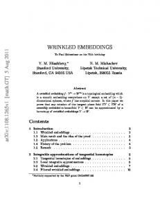
This loss function differs from Eq. (3) in an important way. In Eq. (4), we use a max operation instead of a sum over the negative examples. The main difference between the two formulations is thus the number of negative triplets that affect the loss at each step of stochastic gradient descent (SGD). In Eq. (3), the loss sums the violations across all negatives, while our loss function only considers the penalty incurred by the hardest negative. One way to compare Eq. 3 and Eq. 4 is to consider how they prioritize two typical training examples. Fig. 1 shows two illustrations for typical examples. The positive pair is at the same location in both examples, while the negative samples are at different distances. This illustration shows that while only the hardest negative c0 is important to R@1, the sum loss focuses on moving all the violating negative samples at the same time. Note that since we use SGD to learn our parameters, we take the max over each mini-batch (this is similar to Kiros et al. (2014) who compute the sum in Eq. (3) over the mini-batch). This does not 3

cˆ1 cˆ1 i

cˆ2

c0

cˆ2

c

i

c0

c

cˆ3 cˆ3 Figure 1: An illustration of typical positive pairs and the nearest negative samples. Filled circles show a positive pair (i, c), while empty circles are negative samples for the query i. The dashed circles on the two sides are drawn at the same radii. The example on the left has a higher loss with the sum loss compared to the example on the right. The max loss assigns a higher loss to the example on the right. Notice that the hardest negative example c0 is closer to i in the right example.

give us the hardest negative example in the entire training set but it is effective as long as we get enough violating triplets with non-zero loss. Using sum, there are potentially 2M (M − 1) non-negative terms in the loss, where M is the size of the mini-batch. With max, there will be at most 2M non-negative terms. Note that the set of terms in the sum formulation is always a superset of the set in max. Let us interpret the rank loss in Eq. (3) and compare it with our loss function. Consider a positive pair (i, c) and the set cˆm of all negative samples where i is given as the query. Suppose that the values α + s(i, cˆm ) − s(i, c) follow a normal distribution. Then, [α + s(i, cˆm ) − s(i, c)]+ follows a truncated normal distribution with p · δ(x) at zero, where p is the probability of a negative sample not incurring any penalty. Sampling M − 1 negative samples from this distribution is expected to give us (M − 1)(1 − p) non-negative penalty terms. A generalization of the central limit theorem to the truncated normal distributions (Johnson et al. (1970)) tells us that if there are enough samples, the distribution of the sum of the random variables will be normal. Thus, the sum loss is actually minimizing the mean of the non-negative terms. In doing so, it is aggregating the subtle gradient signal from many samples. Thus the gradient updates are no longer noisy and SGD may not be capable of jumping out of local minima. A similar difficulty is observed when large mini-batches are used for SGD (Goyal et al. (2017)). The max loss reduces the contributing terms and considers only the hardest negatives. While this potentially makes our model more prone to outliers in the training data, we experimentally show that this loss is much more effective on the image-captioning datasets.

4

E XPERIMENTS

We perform experiments with our VSE++ and compare it to the original formulation of Kiros et al. (2014) (referred to as VSE), as well as state-of-the-art approaches. We re-implemented VSE with the help of the authors’ open-source code 2 . For comparison, we present both results and refer to our re-implementation (which improves over the original VSE implementation) as VSE0. We experiment with two image encoders: VGG19 by Simonyan & Zisserman (2014) and ResNet152 by He et al. (2016). Previous works have extracted the image features mostly by pre-computing the FC7 features (the penultimate fully connected layer) of VGG19. We thus explicitly indicate methods that use ResNet152. The dimensionality of the image embedding, Dφ , is 4096 for VGG19 and 2048 for ResNet152. The image features are extracted by first resizing the image to 256 × 256, then using either a single center crop of size 224 × 224 or the mean of feature vectors for 10 crops of similar size as used by Klein et al. (2015) and Vendrov et al. (2015). We refer to training with one center crop as 1C and training with 10 crops as 10C. We also try training using random crops which we denote by RC. For RC, we have the full VGG19 model and extract features over a single randomly chosen cropped patch on the fly as opposed to pre-computing the image features once and reusing them. 2

https://github.com/ryankiros/visual-semantic-embedding

4

#

Model

Trainset

1.1 1.2 1.3 1.4 1.5 1.6 1.7 1.8 1.9 1.10 1.11

VSE (Kiros et al. (2014), GitHub) Order (Vendrov et al. (2015)) Embedding Network (Wang et al. (2017)) sm-LSTM (Huang et al. (2016)) 2WayNet (Eisenschtat & Wolf (2016)) VSE++ VSE++ VSE++ VSE++ (fine-tuned) VSE++ (ResNet152) VSE++ (ResNet152, fine-tuned)

1C (1 fold) 10C+rV ? ? ? 1C (1 fold) RC RC+rV RC+rV RC+rV RC+rV

1.12 1.13 1.14

Order (Vendrov et al. (2015)) VSE++ (fine-tuned) VSE++ (ResNet152, fine-tuned)

10C+rV RC+rV RC+rV

Caption Retrieval Image Retrieval R@1 R@10 Med r R@1 R@10 Med r 1K Test Images 43.4 85.8 2 31.0 79.9 3 46.7 88.9 2.0 37.9 85.9 2.0 50.4 69.4 39.8 86.6 53.2 91.5 1 40.7 87.4 2 55.8 39.7 43.6 84.6 2.0 33.7 81.0 3.0 49.0 88.4 1.8 37.1 83.8 2.0 51.9 90.4 1.0 39.5 85.6 2.0 57.2 93.3 1.0 45.9 89.1 2.0 58.3 93.3 1.0 43.6 87.8 2.0 64.6 95.7 1.0 52.0 92.0 1.0 5K Test Images 23.3 65.0 5.0 18.0 57.6 7.0 32.9 74.7 3.0 24.1 66.2 5.0 41.3 81.2 2.0 30.3 72.4 4.0

Table 1: Results of experiments on MS-COCO. #

Model

Trainset

2.1 1.6 2.2 1.7 2.3 1.8 2.4 1.9 2.5 1.10 2.6 1.11

VSE0 VSE++ VSE0 VSE++ VSE0 VSE++ VSE0 (fine-tuned) VSE++ (fine-tuned) VSE0 (ResNet152) VSE++ (ResNet152) VSE0 (ResNet152, fine-tuned) VSE++ (ResNet152, fine-tuned)

1C (1 fold) 1C (1 fold) RC RC RC+rV RC+rV RC+rV RC+rV RC+rV RC+rV RC+rV RC+rV

Caption Retrieval R@1 R@10 Med r 43.2 85.0 2.0 43.6 84.6 2.0 43.1 87.1 2.0 49.0 88.4 1.8 46.8 89.0 1.8 51.9 90.4 1.0 50.1 90.5 1.6 57.2 93.3 1.0 52.7 91.8 1.0 58.3 93.3 1.0 56.0 93.5 1.0 64.6 95.7 1.0

Image Retrieval R@1 R@10 Med r 33.0 80.7 3.0 33.7 81.0 3.0 32.5 82.1 3.0 37.1 83.8 2.0 34.2 83.6 2.6 39.5 85.6 2.0 39.7 87.2 2.0 45.9 89.1 2.0 36.0 85.5 2.2 43.6 87.8 2.0 43.7 89.7 2.0 52.0 92.0 1.0

Table 2: The effect of various changes to VSE. We copy the relevant results for VSE++ from Table 1 to enable an easier comparison. Notice that applying all the modifications with the exception of the loss function, the VSE model reaches 56.0% for R@1, while VSE++ that employs our proposed loss function achieves 64.6%.

For the caption encoder, we use a GRU similar to the one used in Kiros et al. (2014). We set the dimensionality of the GRU, Dψ , and the joint embedding space, D, to 1024. The dimensionality of the word embeddings that are input to the GRU is set to 300. We further note that in Kiros et al. (2014), the caption embedding is normalized, while the image embedding is not. The normalization of both vectors ensures that the similarity measure is cosine similarity. In VSE++ we normalize both vectors. Not normalizing the image embedding changes the importance of samples and so can be helpful or harmful. In our experiments, not normalizing the image embedding helped the original VSE formulation find a better solution. However, VSE++ is not significantly affected by this normalization. 4.1

DATASETS

We evaluate our method on the Microsoft COCO dataset (Lin et al. (2014b)) and the Flickr30K dataset (Young et al. (2014)). Flickr30K has a standard 30, 000 images for training. Following Karpathy & Fei-Fei (2015), we use 1000 images for validation and 1000 images for testing. We also use the splits of Karpathy & Fei-Fei (2015) for MS-COCO. In this split, the training set contains 82, 783 images, 5000 validation and 5000 test images. However, there are also 30, 504 images that were originally in the validation set of MS-COCO but have been left out in this split. We refer to this set as rV. Some papers use rV for training (113, 287 training images in total) to further improve accuracy. We report results using both training sets. Each image comes with 5 captions. The results are reported by either averaging over 5 folds of 1K test images or testing on the full 5K test images. 5

#

Model R@1

3.1 3.2 3.3 3.4 3.5

Order (Vendrov et al. (2015)) VSE0 Order0 VSE++ Order++

46.7 49.5 48.5 51.3 53.0

Caption Retrieval Image Retrieval R@10 Med r R@1 R@10 Med r 1K Test Images 88.9 2.0 37.9 85.9 2.0 90.0 1.8 38.1 85.1 2.0 90.3 1.8 39.6 86.7 2.0 91.0 1.2 40.1 86.1 2.0 91.9 1.0 42.3 88.1 2.0

Table 3: Comparison on MS-COCO. Training set for all the rows is 10C+rV. 4.2

D ETAILS OF T RAINING

We use the Adam optimizer Kingma & Ba (2014) to train the models. We train most of the models by running 15 epochs with learning rate 0.0002 and then 15 epochs with 0.00002. The fine-tuned models are trained by taking a model that is trained for 30 epochs with a fixed image encoder and then training it for 15 epochs with a learning rate of 0.00002. We set the margin to 0.2 for most of the experiments. We use a mini-batch size of 128 in all our experiments. We do early stopping based on a sum of the recalls on the validation set. We did not see a difference in the performance by changing the mini-batch size if we run for the full 30 epochs. Notice that since the size of the training set for different models is different, the actual number of iterations in each epoch can vary. 4.3

R ESULTS ON MS-COCO

The results on the MS-COCO dataset are presented in Table 1. To ensure transparency with respect to all additional modifications, we report an ablation study for the baseline VSE including these modifications in Table 2. Our best result is achieved by using ResNet152 and fine-tuning the image encoder (row 1.11), where we see 21.2% improvement in R@1 for caption retrieval and 21% improvement in R@1 for image retrieval compared to the original VSE results (row 1.1). Notice that using ResNet152 and fine-tuning can only lead to 12.6% improvement using the original formulation (row 2.6), while our introduced loss function brings a significant gain of 8.6%. Comparing VSE++ (ResNet152, fine-tuned) to the current state-of-the-art on MS-COCO, 2WayNet (row 1.5), we see approximately 8.8% improvement in R@1 for caption retrieval and compared to sm-LSTM (row 1.4), 11.3% improvement in image retrieval. We also report results on the full 5K test set of MS-COCO in row 1.13 and row 1.14. Effect of the training set. We compare VSE and VSE++ by incrementally improving the training data. Comparing the models trained on 1C (row 1.1 and row 1.6), we only see 2.7% improvement in R@1 for image retrieval but no improvement in caption retrieval performance. However, when we train using RC (row 1.7 and row 2.2) or RC+rV (row 1.8 and row 2.3), we see that VSE++ gains an improvement of 5.9% and 5.1%, respectively, in R@1 for caption retrieval compared to VSE0. This shows that VSE++ can better exploit the additional data. Effect of a better image encoding. We also investigate the effect of a better image encoder on the models. Row 1.9 and row 2.4 show the effect of fine-tuning the VGG19 image encoder. We see that the gap between VSE0 and VSE++ increases to 6.1%. If we use ResNet152 instead of VGG19 (row 1.10 and row 2.5), the gap is 5.6%. As for our best result, if we use ResNet152 and also fine-tune the image encoder (row 1.11 and row 2.6) the gap becomes 8.6%. The increase in the performance gap shows that the improved loss of VSE++ can better guide the optimization when a more powerful image encoder is used. 4.4

I MPROVING O RDER E MBEDDINGS

The formulation of Order-embeddings Vendrov et al. (2015), is very similar to VSE with a difference in the similarity measure. Order-embeddings use the asymmetric similarity measure s(i, c) = −k max(0, g(c; Wg , θψ ) − f (i; Wf , θφ ))k2 . Note that, similar to the reported results of order-embeddings, we report the results on the training set 10C+rV. We use the hyper-parameters reported by Order0 to reproduce their results and we get 6

slightly better results (row 3.1 and row 3.3). We use a learning rate of 0.001 for 15 epochs and 0.0001 for another 15 epochs. The margin is set to 0.05. Additionally, Vendrov et al. (2015) takes the absolute value of embeddings before computing the similarity measure. We do not do this in Order++, and stick with our original embedding. We use the same learning schedule and margin as our other experiments. In Table 3, we report the results when replacing the sum loss used in Order-embeddings to our max loss. We can again see that our loss leads to increased performance. We observe 4.5% improvement from Order0 to Order++ in R@1 for caption retrieval (row 3.3 and row 3.5). Compared to the improvement from VSE0 to VSE++, where the improvement on the 10C+rV training set is 1.8%, we gain an even higher improvement here. This shows that our modification can help different methods that use a similar loss function to Eq. (3). 4.5

I NVESTIGATE THE B EHAVIOR OF THE L OSS F UNCTIONS

We investigate the behavior incurred by our loss during training in Figure 2. In particular, we show results during training the VSE and VSE++ with ResNet152 and Order-embeddings using 10C+rV. We notice that our max loss can take a couple of epochs to warm-up. Observe that initially, sum starts off faster, but after approximately 2 epochs max surpasses sum. In order to explain this, notice that the max loss only depends on triplets, rather than a larger set in the case of sum. Since we randomly initialize the parameters, there can be more than one hard negative. However, the gradient of the max loss, will only be influenced by one of them. As such, it can take longer to train a better model than when using the sum loss.

Figure 2: Comparison between the recall performance on the validation set of MS-COCO for the max loss and the sum loss. The left plot compares VSE and VSE++ with ResNet152 as the image encoder with/without fine-tuning (Table 1, row 1.10 and row 1.11 compared to Table 2, row 2.5 and row 2.6). The right plot compares the two formulations for Order-embeddings (Table 3, row 3.3 and row 3.5). Notice that for Order-embeddings, in the first 2 epochs the original loss function achieves a better performance, however, from there-on our loss function leads to much higher recall rates.

4.6

R ESULTS ON F LICKR 30K

We report the results on the Flickr30K dataset in Tables 4.1 and 4.13. Here, we obtain 23.1% improvement in R@1 for caption retrieval and 17.6% improvement in R@1 for image retrieval (row 4.1 and row 4.13). Since the size of the Flickr30K training data is small, we observed that VSE++ overfits when the pre-computed features of a single center crop is used. We do early stopping to stop before over-fitting happens. We run for a fixed number of epochs and save checkpoints at the end of each epoch. The checkpoint with the maximum sum of the recalls on the validation set is taken as the best model for comparison to other models. The over-fitting is resolved when the model is trained using RC. Our results show that the improvements incurred by our simple modification to the loss function persists across datasets, as well as across models. These are drastic improvements, and we hope to see similar behavior on other tasks in the future. 7

#

Model

Trainset

4.1 4.2 4.3 4.4 4.5 4.6 4.7 4.8 4.9 4.10 4.11 4.12 4.13

VSE (Kiros et al. (2014)) VSE (GitHub) Embedding Network (Wang et al. (2017)) DAN (Nam et al. (2016)) sm-LSTM (Huang et al. (2016)) 2WayNet (Eisenschtat & Wolf (2016)) DAN (ResNet152) (Nam et al. (2016)) VSE0 VSE++ VSE++ VSE++ (fine-tuned) VSE++ (ResNet152) VSE++ (ResNet152, fine-tuned)

1C 1C ? ? ? ? ? 1C 1C RC RC RC RC

Caption Retrieval R@1 R@10 Med r 23.0 62.9 5 29.8 70.5 4 40.7 79.2 41.4 82.5 2 42.5 81.5 2 49.8 55.0 89.0 1 29.8 71.9 3.0 31.9 68.0 4.0 38.6 74.6 2.0 41.3 77.9 2.0 43.7 82.1 2.0 52.9 87.2 1.0

Image Retrieval R@1 R@10 Med r 16.8 56.5 8 22.0 59.3 6 29.2 71.7 31.8 72.5 3 30.2 72.3 3 36.0 39.4 79.1 2 23.0 61.0 6.0 23.1 60.7 6.0 26.8 66.8 4.0 31.4 71.2 3.0 32.3 72.1 3.0 39.6 79.5 2.0

Table 4: Results on the Flickr30K dataset.

VSE0: [9] Three elephants kick up dust as they walk through the flat by the bushes.

VSE0: [1] A party decoration containing flowers, flags, and candles.

VSE0: [24] A person standing on a skate board in an alley.

VSE0: [2] a parking area for motorcycles and bicycles along a street

VSE++: [1] A couple elephants walking by a tree after sunset.

VSE++: [1] A party decoration containing flowers, flags, and candles.

VSE++: [10] Two young men are skateboarding on the street.

VSE++: [1] A number of motorbikes parked on an alley

VSE0: [39] Young skateboarder displaying skills on sidewalk near field.

VSE0: [6] A large slice of angel food cake sitting on top of a plate.

VSE0: [1] A woman holding a child and standing near a bull.

VSE0: [6] A man playing tennis and holding back his racket to hit the ball.

VSE++: [3] Two young men are outside skateboarding together.

VSE++: [16] A baked loaf of bread is shown still in the pan.

VSE++: [1] A woman holding a child looking at a cow.

VSE++: [1] A woman is standing while holding a tennis racket.

Figure 3: Examples of test images and the top 1 retrieved captions for VSE0 and VSE++ (ResNet)finetune. The value in brackets is the rank of the highest ranked ground-truth caption.

5

C ONCLUSION

In this paper, we focused on the task of image-caption retrieval and investigated visual-semantic embeddings. We have shown that a new loss function that uses only violation incurred by hard negatives drastically improves performance over the typical loss that sums the violations across the negatives, typically used in previous work (Kiros et al. (2014); Vendrov et al. (2015)). We performed experiments on the MS-COCO and Flickr30K datasets. We observed that the improved loss can better guide a more powerful image encoder, ResNet152, and also guide better when fine-tuning an image encoder. With all modifications, our VSE++ model achieves state-of-the-art performance on the MS-COCO dataset, and is slightly below the best recent model on the Flickr30K dataset. Our proposed improvement can be used to train more sophisticated models that have been using a similar rank loss for training. 8

R EFERENCES Eisenschtat, Aviv and Wolf, Lior. arXiv:1608.07973, 2016. 2, 5, 8

Linking image and text with 2-way nets.

arXiv preprint

Goyal, Priya, Doll´ar, Piotr, Girshick, Ross, Noordhuis, Pieter, Wesolowski, Lukasz, Kyrola, Aapo, Tulloch, Andrew, Jia, Yangqing, and He, Kaiming. Accurate, large minibatch sgd: Training imagenet in 1 hour. arXiv preprint arXiv:1706.02677, 2017. 4 He, Kaiming, Zhang, Xiangyu, Ren, Shaoqing, and Sun, Jian. Deep residual learning for image recognition. In IEEE CVPR, pp. 770–778, 2016. 2, 4 Hodosh, Micah, Young, Peter, and Hockenmaier, Julia. Framing image description as a ranking task: Data, models and evaluation metrics. Journal of Artificial Intelligence Research, 47:853– 899, 2013. 2 Huang, Yan, Wang, Wei, and Wang, Liang. Instance-aware image and sentence matching with selective multimodal lstm. arXiv preprint arXiv:1611.05588, 2016. 2, 5, 8 Johnson, Norman L, Kotz, Samuel, and Balakrishnan, N. Distributions in statistics: continuous univariate distributions, vol. 2. NY: Wiley, 1970. 4 Karpathy, Andrej and Fei-Fei, Li. Deep visual-semantic alignments for generating image descriptions. In IEEE CVPR, pp. 3128–3137, 2015. 1, 2, 3, 5 Kingma, Diederik and Ba, Jimmy. Adam: A method for stochastic optimization. arXiv preprint arXiv preprint arXiv:1412.6980, 2014. 6 Kiros, Ryan, Salakhutdinov, Ruslan, and Zemel, Richard S. Unifying visual-semantic embeddings with multimodal neural language models. arXiv preprint arXiv:1411.2539, 2014. 1, 2, 3, 4, 5, 8 Klein, Benjamin, Lev, Guy, Sadeh, Gil, and Wolf, Lior. Associating neural word embeddings with deep image representations using fisher vectors. In IEEE CVPR, pp. 4437–4446, 2015. 1, 2, 4 Lin, Dahua, Fidler, Sanja, Kong, Chen, and Urtasun, Raquel. Visual Semantic Search: Retrieving Videos via Complex Textual Queries. IEEE CVPR, 2014a. 2 Lin, Tsung-Yi, Maire, Michael, Belongie, Serge, Hays, James, Perona, Pietro, Ramanan, Deva, Doll´ar, Piotr, and Zitnick, C Lawrence. Microsoft coco: Common objects in context. In ECCV, pp. 740–755. Springer, 2014b. 5 Malinowski, Mateusz, Rohrbach, Marcus, and Fritz, Mario. Ask your neurons: A neural-based approach to answering questions about images. In ICCV, 2015. 1 Nam, Hyeonseob, Ha, Jung-Woo, and Kim, Jeonghee. Dual attention networks for multimodal reasoning and matching. arXiv preprint arXiv:1611.00471, 2016. 2, 8 Simonyan, Karen and Zisserman, Andrew. Very deep convolutional networks for large-scale image recognition. arXiv preprint arXiv:1409.1556, 2014. 2, 4 Socher, Richard, Karpathy, Andrej, Le, Quoc V, Manning, Christopher D, and Ng, Andrew Y. Grounded compositional semantics for finding and describing images with sentences. Association for Computational Linguistics (ACL), 2:207–218, 2014. 2, 3 Vendrov, Ivan, Kiros, Ryan, Fidler, Sanja, and Urtasun, Raquel. Order-embeddings of images and language. arXiv preprint arXiv:1511.06361, 2015. 1, 2, 4, 5, 6, 7, 8 Wang, Liwei, Li, Yin, and Lazebnik, Svetlana. Learning two-branch neural networks for image-text matching tasks. arXiv preprint arXiv:1704.03470, 2017. 2, 5, 8 Young, Peter, Lai, Alice, Hodosh, Micah, and Hockenmaier, Julia. From image descriptions to visual denotations: New similarity metrics for semantic inference over event descriptions. Association for Computational Linguistics (ACL), 2:67–78, 2014. 5 Zhu, Yukun, Kiros, Ryan, Zemel, Rich, Salakhutdinov, Ruslan, Urtasun, Raquel, Torralba, Antonio, and Fidler, Sanja. Aligning books and movies: Towards story-like visual explanations by watching movies and reading books. In ICCV, 2015. 1, 2 9