Characterisation and Source Apportionment of Submicron Particle ...

Aerosol and Air Quality Research, 15: 220–233, 2015 Copyright © Taiwan Association for Aerosol Research ISSN: 1680-8584 print / 2071-1409 online doi: 10.4209/aaqr.2014.06.0108

Characterisation and Source Apportionment of Submicron Particle Number Size Distributions in a Busy Street Canyon Patricia Krecl1*, Admir Créso Targino1, Christer Johansson2,3, Johan Ström2 1

Federal Technological University of Paraná, Graduate Program in Environmental Engineering, Apucarana-Londrina, Brazil 2 Department of Applied Environmental Science (ITM), Stockholm University, Stockholm, Sweden 3 Stockholm Environment and Health Administration, Stockholm, Sweden ABSTRACT Street canyons are well-known hot spots due to the harmful exposure to high concentrations of atmospheric pollutants emitted mainly by motor vehicles. We report on measurements of air pollutants conducted in a street canyon in Stockholm (Sweden) in spring 2006. Particle number size distributions (PNSD) were measured in the 25–606 nm range, along with total particle number, light-absorbing carbon mass concentration (MLAC), PM10, NOx, CO, traffic rate (TR), vehicle speed and meteorological variables. We used PNSD as input to the positive matrix factorisation (PMF) analysis to identify and apportion the pollutant sources. All pollutants showed distinct diurnal patterns, with highest concentrations in weekday mornings (08:00–09:00). TR was always higher on weekdays, except for the early hours (00:00–06:00). The raise in the weekend early-hour TR was accompanied by the largest MLAC of the day, a higher NOx/CO ratio compared to weekdays and a modal shift of PNSD towards larger diameters (47–56 nm), indicates a change in the vehicle fleet share to being dominated by diesel-run taxis. The largest contribution to the submicron particles was observed for winds blowing along the canyon, transporting particles emitted by vehicles accelerating from the traffic lights at the intersection, uphill towards the measurement site, and from the nearby streets. Three PMF factors were identified: local emissions from a mixed fleet dominated by gasoline engines, local traffic emissions highly impacted by diesel vehicles, and urban background aerosol. On average, gasoline-fuelled vehicles largely contributed to NOx, and particle number concentrations (54–65%), whereas MLAC sources were dominated by diesel emissions, especially at weekends in the early hours (73%). The urban background contribution was rather low (4–13%) and with little dependence on the weekday. This work demonstrated how particle size distribution measurements, together with MLAC, NOx and CO can be used to quantify the contribution from diesel and gasoline vehicles. Keywords: DMPS; Traffic emissions; PMF; Urban air quality; Black carbon.

INTRODUCTION Within the urban canopy layer, street canyons have been the subject of active research due to their complex air flow patterns (Carpentieri et al., 2009 and references therein) and temperature gradients that contribute to the development of urban heat islands (e.g., Memon and Leung, 2011). From the air pollution viewpoint, street canyon micro-environments are of particular interest because they present elevated concentration of pollutants due to high traffic emissions and limited local dispersion conditions. For example, measurements conducted in cities across Europe showed

*

Corresponding author. Tel.: +55-43-3162-1200 E-mail address: [email protected]

that air quality standards for particulate matter concentrations (PM10 and PM2.5) are exceeded at kerbside stations, and especially in canyon configurations (Putaud et al., 2010). Since street canyons are mostly located in the inner city, where population and traffic densities are high, a great fraction of the urban residents is exposed to harmful atmospheric pollutants on a daily basis and experience higher mortality and morbidity risks (Forsberg et al., 2005). Also drivers, cyclists and pedestrians occupying those streets may receive, in a short period of time, a significant dose of their daily total exposure (Boogaard et al., 2009). The effect of atmospheric particles on human health is usually linked to mass concentration measurements expressed as PM10 or PM2.5. Even though there is a large body of epidemiological and toxicological studies associating the exposure to submicron particles with detrimental health effects, particle number and size distribution concentrations –which are important metrics of toxic aerosols– are still not

Krecl et al., Aerosol and Air Quality Research, 15: 220–233, 2015

directly regulated. Ultrafine particles –a fraction of submicron particles, with aerodynamic diameter less than 100 nm– have been associated with a series of health problems, such as premature death, aggravated asthma and chronic bronchitis (e.g., Asgharian and Price 2007; Murr and Garza, 2009). In urban environments, the contribution of road traffic emissions to the number concentration of ultrafine particles is dominant (e.g., Johansson et al., 2007), because particles generated from gasoline and diesel combustion are mainly smaller than 60 nm and 100 nm, respectively (Kittelson, 1998; Gouriou et al., 2004). Diesel-powered vehicles, which are usually a smaller fraction of the fleet, make a proportionally large contribution to total number concentrations (Kittelson et al., 2006b). Contributions from gasoline-fuelled vehicles are highly dependent on driving conditions, and are much higher during acceleration, at high vehicle speed (VS), and during cold starts (Kittelson et al., 2006a). Besides vehicle fleet composition and traffic conditions, PNSD are influenced by meteorological conditions, longrange transport and the city’s attributes, such as the configuration of urban canyons, which affect both concentration levels and the shape of the distribution curves. Thus, developing a proper air pollution regulatory framework requires the characterisation of the submicron fraction of airborne particles to aid in determining their emission sources, particularly in hot-spot areas. Whilst urban aerosols properties, such as number and mass concentrations and chemical composition, have been extensively addressed, data characterising the PNSD (especially in urban canyons) are relatively sparse (Ketzel et al., 2003; Longley et al., 2003). We conducted this work in a street canyon in Stockholm, which is the largest metropolitan region in Scandinavia with a population of 1.25 million inhabitants. We focus on PNSD and use auxiliary measurements of other atmospheric pollutants (total number concentration, PM10, MLAC, NOx and CO), traffic data and meteorology to help characterise their emission sources. Because WS and cross- or alongcanyon WD are the most important factors influencing the flow, mixing processes and the pollutant concentrations in street canyons (Ketzel et al., 2003; Vardoulakis et al., 2003), we also investigated the influence of these variables on PNSD, particle mass and gas concentrations. Then, hourly mean PNSD were analysed using the positive matrix factorisation (PMF) method to identify and apportion the emission sources. METHODS Experimental Set-up The sampling site was located in central Stockholm in a regular (height-to-width ratio of 1) street canyon on Hornsgatan road (see Gidhagen et al. (2004a) for a canyon layout). This street transect is situated roughly in the westeast direction (255 degrees from the North) with 24-m height buildings flanking both sides of the road, and only 67 m west of Ringvägen street –another highly trafficked street (~13,000 vehicles per day). The daily mean traffic rate (TR) on Hornsgatan is ~30,700 vehicles on weekdays (~23,400

221

at weekends), organised in four lanes (two lanes for each direction) with a speed limit of 50 km h–1, and controlled by a traffic light situated at the intersection with Ringvägen street. Frequent congestions, start-stop driving, as well as acceleration and deceleration (hill slope of 2.3%) are usually observed. Automatic number plate recordings of four million vehicles showed that on average, the composition of the vehicle fleet is: passenger cars 77%, light-duty vehicles 12%, buses 2%, and heavy-duty vehicles 1%. Half of the vehicle fleet runs on gasoline, 30% uses diesel (21% of the passenger cars, most of the taxis and heavy-duty vehicles), and 14% are ethanol vehicles (80% of the buses and 15% of the passenger cars) (Burman and Johansson, 2010). Instruments were housed in a trailer parked on the northern side of the road (lat: 59.317 N, lon: 18.049 E) and measurements were conducted in the period 11 April–20 June 2006. The height of the sampling inlets varied between 2.5 and 3.7 m above the ground. Particle number size distributions were measured in the 25–606 diameter range using a custom-built differential mobility particle sizer (DMPS) described elsewhere (e.g., Krecl et al., 2008). The flow rates were set to 1.5 and 5.5 L min–1 for the aerosol and sheath flows, respectively. The scanning time for each spectrum was 2 minutes, using alternating up-and down scans. The inversion algorithm considered the charging efficiency as a function of the particle diameter and a correction for double charges was applied (Wiedensholer, 1988). The particle number concentration in the diameter range 25–606 nm (N25-606) was calculated by integrating the particle number size distribution. The particle number concentration was also measured using a CPC (model TSI 3022, TSI Inc., USA) with a lower cut-off size of 7 nm (N7). PM10 mass concentrations were monitored by an automatic Tapered Element Oscillating Microbalance (TEOM 1400a, Rupprecht & Patashnick Inc., USA) with heated inlets (50°C) to avoid condensing water, and were corrected to account for losses of volatile material on the particles (Krecl et al., 2011). Measurements of MLAC were carried out by a custombuilt Particle Soot Absorption Photometer (PSAP) and several corrections were applied as described in Krecl et al. (2011). NOx and CO were simultaneously monitored on the northern and southern sides of the road with a commercial chemiluminescence analyser (model 31 M LCD, Environment SA, France) and an automatic infrared-absorption CO analyser (Thermo Scientific, model 48i with Ndir technology). Zero and the span of the gas instruments were checked daily, and the analysers were calibrated every 1–2 months. Traffic stream data (TR and VS) were recorded using an automatic Marksman loop counter, model 660 (Golden River Traffic Ltd., UK). Road wetness was monitored using a simple electrical resistance wire (custom-built) installed at 5.1 m from the kerbside. Meteorological measurements were conducted on a rooftop platform (25 m height), located 450 m southeast of Hornsgatan site, including air temperature (Hygroclip probe, Rotronic AG, Switzerland), precipitation (tipping bucket rain gauge, model HB 3166-06, Casella Measurement, UK), and wind (ultrasonic anemometer, model R3, Gill Instruments Ltd., UK). The sensors were installed at 2 m above roof

Krecl et al., Aerosol and Air Quality Research, 15: 220–233, 2015

222

level, except for the anemometer installed at 10 m above the roof. Concurrent PM10, MLAC and NOx measurements were also conducted at this rooftop platform and are described elsewhere (Krecl et al., 2011). All data are reported in local standard time (UTC + 1). PMF Analysis We used PNSD as input to the PMF2 algorithm (YPTekniika KY company, Finland) to identify and apportion the pollutant sources in the street canyon. PMF is a multivariate least-squares technique that constrains the solution to be non-negative and takes into account the uncertainty of the observed data (Paatero and Tapper, 1994). The basic source-receptor model in matrix form is: X = G.F + E,

(1)

where X is the observed PNSD matrix, G and F are, respectively, the source contributions and PNSD profiles of the unknown sources to be estimated from the analysis, and E is the residual matrix (observed - estimated). Eq. (1) can also be expressed in the element form as: p

xij   gik  f kj  e ij ,

(2)

k 1

where xij is the particle number concentration of size interval j measured on sample i, p is the number of factors contributing to the samples, fkj is the concentration of size bin j from the kth factor, gik is the relative contribution of factor k to sample i, and eij is the residual value (estimated - observed) for the size bin j measured on the sample i. For a given p, values of fkj and gik are adjusted using a leastsquare method (with the constraint that fkj and gik values are non-negative), until a minimum Q value is found:

 eij Q   i 1 j 1    ij n

m

2

  , 

(3)

where σij is the uncertainty of the particle number concentration of size bin j in sample i, n is the number of samples, and m is the number of size intervals. In this study, we applied PMF on hourly PNSD with n = 1011, and m = 16. The methodology applied to produce a PMF solution included the following steps: i) determining the model parameters: number of factors, the Fpeak parameter that controls the rotational freedom of the solutions, error model, PMF mode and outliers influence, ii) running the PMF model, and checking the solution convergence to a global minimum, iii) assessing the goodness of the model fit, and iv) estimating the model uncertainties. Different factor numbers were tested and a 3-factor model adequately fitted the data with the most meaningful results. When 4 factors were included in the analysis, no more relevant sources could be identified. To determine the optimal values for the Fpeak parameter, we analysed the linear correlation between factor contributions from the

PMF analysis against each other for Fpeak values ranging from –2 to +2 in steps of 0.1 (Paatero et al. 2005). The lowest correlation coefficient (R) was found for Fpeak = –0.9, indicating the minimum statistical independence between pairs of g-factors. A dynamical error model was chosen for this study and PMF uncertainties σij were calculated at each iteration step of the program by using: σij = Cij + C3 max(|xij|, |yij|),

(4)

where Cij is the measurement error, C3 is a constant value that accounts for some source profile variation -giving the fitting more flexibility to accommodate this variability-, and max(|xij|, |yij|) is the maximum value between the observed xij and the modelled yij. Since the DMPS measurement errors in size and number were quite small (2–3%), we set up Cij to 0 and included all the uncertainty input in the C3 constant. In order to obtain small scaled residuals, C3 was set up to 0.25. PMF was run in the robust mode to reduce the influence of atypical measurements in the dataset and three values of the outlier threshold distance α were tested: 2, 4, and 8. Because α = 4 and α = 8 yielded similar scaled residuals in the range [–2.3, 3.0], we ran PMF with α = 4. The model uncertainty was estimated by randomly removing 25% of the original samples and then running the PMF model 300 times on these new datasets (Krecl et al., 2008). We considered the PMF solution stable since the difference between the mean factor profiles after removing 25% of the samples, and the factor profiles –when all samples (using the same model initialization values) were included– lay between one standard deviation values. The PMF solution converged and a global minimum was found in 5 runs using different pseudo-random seeds. Moreover, the same output values (f and g-factors, and Q) were found for all the runs. Then, the emission sources were identified based on the profiles of the f-factors by searching the literature for measurements of PNSD with similar characteristics, analysing the diurnal variation of the modelled concentrations, and correlating the factor contributions and observed concentrations. Finally, a multiple linear regression model (MLR) of the g-factors onto the measured concentrations of each aerosol and trace gas variable was performed (Krecl et al., 2008). The MLR model expresses the concentrations of each variable as a linear function of the g-factors and determines the regression coefficients and their confidence intervals (95%). The goodness of the model fit was assessed by comparing the modelled and observed concentrations for each trace gas and aerosol variables, and analysing whether the residual concentrations were normally distributed. The source contributions to each variable were estimated with the calculated regressions coefficients. RESULTS AND DISCUSSION General Overview During the field campaign, the long-range transport of pollutants emitted by agricultural wildfires in western Russia and the Baltic region deteriorated the air quality in

Krecl et al., Aerosol and Air Quality Research, 15: 220–233, 2015

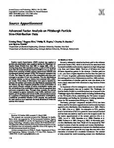
Northern Europe, causing record high pollution levels as far as the Arctic (Treffeisen et al., 2007). In the period 24 April–9 May 2006, Targino et al. (2013) observed enhanced concentrations of elemental and organic carbon, PM2.5 and O3, together with a 200% increase in the particle number accumulation mode (100–450 nm range) at urban background and kerbside stations in Stockholm. This was an exceptional long-range transport event, and we excluded concurrent measurements from our analysis to focus on typical pollution conditions in the street canyon. Daily mean temperatures ranged between 3.7°C and 23.6°C, and relative humidity in the range 39–91%. The mean wind speed (WS) at rooftop was 3.6 m/s and the prevailing wind directions (WD) were south (23%), west (23%), and southwest (22%) (Figs. 4(e) and 4(f)). Precipitation was observed on 16 of 43 days and daily accumulated values were always lower than 10 mm. Due to the location of our site, we expected a large influence of road traffic emissions on concentrations of atmospheric pollutants. Thus, the data were classified as weekday (Mon–Fri, 28 days) or weekend (Sat–Sun and red days, 15 days). Descriptive statistics showed a large variability in all aerosol and trace gas concentrations on weekdays and weekends (Table 1). For all variables analysed, weekday levels were higher than weekend concentrations (on average 1.2–1.5 times higher). Assuming that particles larger than 606 nm (the upper cutoff of the DMPS) make up a little fraction of the total particle number concentration in urban areas (Morawska et al., 1998), we calculated the contribution of the smallest particles (7–25 nm) to the total number concentration by subtracting N25-606 from N7 (no particular corrections for inlet losses or instrumentation detection efficiencies were applied). The contribution both on weekdays and at weekends was ~73%, which reinforces other studies that show that road vehicles are a major emission source of ultrafine particles (Johansson et al., 2007; Shi et al., 2001). Regardless of the day of the week, the mean contribution of MLAC to PM10 was 11%. Particle Number Size Distributions Fig. 1 shows the mean diurnal evolution of the PNSD (Figs. 1(a) and 1(b)), together with mean profiles for selected

223

times of the day (Figs. 1(c) and 1(d)) for weekdays and weekends. The upper panels reflect the traffic pattern in an urban environment, with increase in concentrations in the morning and evening rush hours, a moderate decrease during the day, and low values during the nighttime. Minimum particle number concentrations occurred in the early morning on weekdays (05:00–06:00) and weekends (06:00–07:00) when TR was low in the canyon (~230 vehicles h–1, Fig. 2(g)). The highest particle number concentrations occurred on weekdays between 08:00 and 09:00 (3.8 × 104 cm–3 at 28 nm) when TR reached ~2,000 vehicles h–1. A secondary maximum of 3.0 × 104 cm–3 (at 28 nm) was observed between 16:00 and 17:00 when TR mounted to 2,200 vehicles h–1. During weekends, not only were the concentrations lower, but the difference between nighttime and daytime maxima was reduced. Peak concentrations were found later than on weekdays (11:00–18:00), concurrent with the highest TR at weekends (~1600 vehicles h–1). The aerosol mode diameter shifted throughout the day (Figs. 1(c) and 1(d)); for weekdays, evening distributions presented larger peak diameters (33– 40 nm, for example at 01:00) whilst smaller sizes (28 nm) were found the rest of the day. The concentrations seemed to peak at diameters smaller than 28 nm, but we could not observe this mode due to the lower cut-off of the DMPS. At weekends during daytime, the maximum particle concentration occurred in the same size range as weekdays (28 nm, for example, at 13:00). On the other hand, the mode shifted and remained around 47–56 nm between 00:00 and 07:00. This almost constant peak diameter in the early hours suggests that the source of particles remained unchanged, producing size distributions very similar in shape, only varying in the number concentration. Ketzel et al. (2003) also observed this pattern in Copenhagen during nighttime at weekends and attributed it to the higher diesel-driven taxi share at weekends. The structure of the PNSD seems to reflect the fact that the Hornsgatan site was dominated by gasoline- and dieselvehicle emissions. Revising the literature, the first peak (< 30 nm) is mainly attributed to carbonaceous particles directly emitted by gasoline emissions, and homogeneous nucleation from the supersaturation of semivolatile precursors due to the rapid cooling of both gasoline and diesel traffic

Table 1. Descriptive statistics of hourly aerosol and trace gas concentrations for weekdays and weekends. Statistics

Day

Arithmetic mean

Weekday Weekend Weekday Weekend Weekday Weekend Weekday Weekend Weekday Weekend Weekday Weekend

Median 5th percentile 95th percentile Standard deviation # samples

PM10 [µg m–3] 49.3 34.2 38.1 27.2 11.0 10.3 138.6 89.9 40.2 25.0 836 480

MLAC [µg m–3] 5.3 3.6 4.6 2.9 1.4 1.3 11.6 8.5 3.2 2.2 787 454

NOx [µg m–3] 128.0 86.9 114.7 75.3 23.6 24.7 286.8 182.2 84.2 50.7 814 480

CO [mg m–3] 0.54 0.47 0.51 0.41 0.21 0.20 1.00 0.92 0.26 0.23 835 480

N7 [cm–3] 45,958 31,721 42,868 29,269 13,379 11,870 91,121 60,383 24,870 15,246 766 449

N25-606 [cm–3] 12,021 8,727 10,636 7,418 3,889 3,868 24,748 17,101 6,679 4,266 660 351

Krecl et al., Aerosol and Air Quality Research, 15: 220–233, 2015

224

WEEKEND

WEEKDAY 7 6 5 4

a

b

3

p

D [nm]

2

100 7 6 5 4 30 0

6

12 Local time (start)

18

23 0

6

12 Local time (start)

18

23

dN/dlogD [cm−3] 0

10000

20000

30000

40000

p

4 01:00 05:00 08:00 13:00

3

d

p

4

−3

dN/dlogD [10 cm ]

c

2

1

0 1 10

2

10 D [nm] p

3

1

10 10

2

10 D [nm]

3

10

p

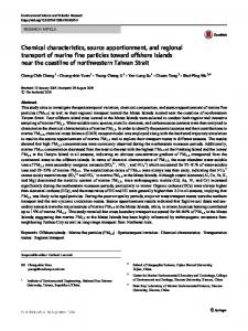
Fig. 1. Hourly mean PNSD on weekdays (left) and weekends (right) for selected times of the day (a, b: start time) and diurnal evolution (c, d) at Hornsgatan site. exhaust gas (e.g., Imhof et al., 2005b). The second peak (50–100 nm) is indicative of diesel emissions, mainly soot aggregates from incomplete combustion processes (Imhof et al., 2005a). Ntziachristos et al. (2007) found a mode at 70– 80 nm in the proximity of freeways with high composition of diesel traffic in Los Angeles. Gouriou et al. (2004) also reported a mode between 60 and 100 nm, which corresponds to emissions from diesel vehicle idling at traffic lights or driving up a slope (higher engine loads). Kittelson et al. (2006b) measured peak concentrations between 52 to 62 nm when chasing diesel vehicles on road, and also a nuclei mode from 6 to 11 nm as a result of the cooling of volatile precursors as the exhaust dilutes. To further investigate the modal shift at Hornsgatan site, we study in the next subsection the diurnal variation of other atmospheric co-pollutants. Diurnal Pattern of Co-pollutants Since diesel and gasoline vehicles were not counted separately, we used other air pollution variables to help characterise the PNSD and disentangle the contribution from each category. Fig. 2 shows the mean diurnal variation of several aerosol and trace gas concentrations, TR and VS for weekdays and weekends at Hornsgatan site. As depicted

in Fig. 1 for PNSD, the traffic emissions impact air pollutants differently on weekdays and weekends. Despite higher TR in the afternoon of weekdays, peak concentrations were observed in the morning, but for PM10, which showed large concentrations between about 06:00 and 15:00. This early morning pattern may be associated with well-documented decay of the mixing layer in the evening and morning, whilst the growth of the mixing layer in the afternoon facilitates a more effective dilution of the pollutants. The concentrations were significantly higher in daytime of weekdays compared to weekends (a Mann-Whitney U test was performed at 95% confidence level) as follows: 1) MLAC, NOx, N7, and N25-606 between 06:00 and 18:00 LT, 2) PM10 concentrations between 06:00 and 12:00), and 3) CO levels in the early morning (06:00–09:00). Daily mean PM10 mass concentrations exceeded the air quality standards (> 50 µg m–3) on 16 days in the studied period (excluding the LRT event) in connection to dry road surface conditions, use of studded tires and high TR both on weekdays (06:00–18:00) and at weekends (11:00–18:00). Johansson et al. (2007) also observed large PM10 mass concentrations in Stockholm and reported that up to 90% of the PM10 mass is due to road abrasion and dust resuspension

Krecl et al., Aerosol and Air Quality Research, 15: 220–233, 2015 9

2

b [104 cm−3]

weekday weekend

1.5

1

25−606

6

3

N

7

N [104 cm−3]

a

0 80

0.5

0 10

d

c 8

MLAC [μg m ]

60 −3

−3

[μg m ]

225

PM

10

40

20

6 4 2

0

0 0.9

f

e CO [mg m−3]

−3

NOx [μg m ]

200

100

0

h

60

g VS [km h−1]

−1

0.3

0

2000

TR [vehicle h ]

0.6

1500 1000

40

weekday, westbound weekday, eastbound weekend, westbound weekend, eastbound

20

500 0

0 0

6

12 18 Time of day (start)

23

0

6

12 18 Time of day (start)

23

Fig. 2. Average diurnal variation of several aerosol and trace gas concentrations, TR and VS for weekdays and weekends. Eastbound side indicates driving towards the city centre. caused by the use of studded tires in winter and early spring. The CO concentrations presented a distinct behaviour compared to the other pollutants, with a well-defined peak between 07:00 and 09:00 on weekdays. Kristensson et al. (2004) reported high CO concentrations inside a road tunnel in Stockholm between 08:00 and 10:00, matching a traffic peak of light-duty vehicles driving at relatively low speeds (40–80 km h–1) and large emission factors for CO were found at low speed intervals (9 g km–1 at 45 km h–1). In our case, the morning CO peak coincides with low VS (mean of 33 km h–1, Fig. 2(h)), especially for vehicles driving

into the city centre, on the eastbound lane which slopes downwards up to the traffic lights. Thus, the CO maximum can be associated with a synergistic effect of increase in emissions by gasoline-vehicle, reduced vehicle speed and poor mixing in the canyon. Increased traffic volume and lower vehicle speed caused a secondary CO peak at about 17:00, which was alleviated by more efficient dispersion in the canyon. In the early hours (00:00–06:00) during weekends, the MLAC concentrations were largest and significantly higher than on weekdays (Mann-Whitney U test at 95% confidence

Krecl et al., Aerosol and Air Quality Research, 15: 220–233, 2015

226

level). This outstanding feature concurred with an increase in NOx levels and TR (especially diesel taxis identified by automatic number plate recordings described by Burman and Johansson, 2010), constant CO levels, decrease in the number concentration of very small particles (7–25 nm) and the modal shift of PNSD towards larger particles (Fig. 1(d)). We can conclude that in the early hours at weekends exhaust particles and trace gases inside the canyon were mainly emitted by diesel vehicles. Correlation Analysis There is a high and positive linear correlation between hourly MLAC, N25-606, NOx, and N7 on weekdays, which is associated with these pollutants originating to a large extend from traffic exhaust emissions (Table 2). At weekends, the correlation between MLAC and NOx was lower (0.78 vs. 0.61) and the correlation between CO and NOx, and CO and N7 increased, suggesting a change in the exhaust emissions. Regardless the day of the week, TR and VS were highly anti-correlated, and PM10 mass concentrations presented rather low correlation with all variables due to the large non-exhaust contribution. Fig. 3 displays the linear correlation coefficient R between hourly air pollutant concentrations and particle number concentration per channel, for weekdays and weekends. In general, correlations were highest on weekdays when traffic dominated the emission sources (on average, 32% more vehicles were counted on weekdays). On weekends, when traffic emissions were lower, other emission sources contributed with a larger fraction of aerosols in the accumulation mode than on weekdays. Correlations between N7 and dN/dlogDp (Fig. 3(a)) and between N25-606 and dN/dlogDp (Fig. 3(b)) showed a similar pattern, with the highest correlation at Dp ~47 nm, and correlations between N7 and dN/dlogDp and N25-606 and dN/dlogDp dropped dramatically for particles larger than 100 and 200 nm, respectively. N7 was dominated by ultrafine particles and its correlation with accumulation mode particles was higher on weekdays (when particles were traffic-dominated) than on weekends (when the contribution of other emission sources to the accumulation mode particles was larger). Because freshly emitted ultrafine particles contributed less to the N25-606 data and to the dN/dlogDp concentrations in the size range 25–606 nm, the correlation between N25-606 and dN/dlogDp was very similar on weekdays and weekends. In the case of PM10 mass concentrations, the correlation is

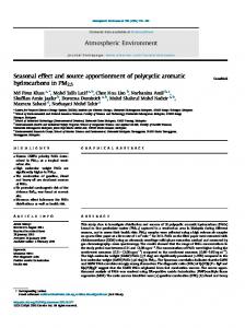
low (|R| < 0.50) for all particle diameters and days of the week. This reinforces the idea that the particles that largely contributed to PM10 mass had a different origin than the submicron particles observed in the canyon. MLAC concentrations were highly correlated (R > 0.75) with number concentration of particles in the range 56–119 nm irrespective of the weekday. The maximum correlation (R = 0.87) was found at Dp ~113 nm, similar to the diameter found in Santiago de Chile (Dp ~100 nm) (G. Olivares, personal communication, 2014) which coincides with the strong unimodal diameter of elemental carbon mass distribution emitted by automobiles (Ning et al., 2013). Correlations between NOx and number concentration per channel were generally higher (Fig. 3(e)) than correlations between CO and dN/dlogDp (Fig. 3(f)), since NOx is usually a better tracer for fresh traffic emissions than CO. On average at Hornsgatan site, concentrations of CO and NOx at street level were 2.0 and 5.5 times higher than at rooftop (not shown), respectively, indicating other important emission sources of CO than traffic. As submicron particle number concentrations in cities are dominated by traffic contributions (e.g., Kumar et al., 2010), it is expected that correlations between NOx levels and number concentration per channel are higher than when CO is correlated with dN/dlogDp. Particles between 56 and 119 nm were highly correlated with NOx on weekdays when vehicle exhaust dominated the emission sources (Fig. 3(f)). Rooftop Wind Influence Rooftop winds blowing perpendicular to the street or with directions to the street axis exceeding 30° and WS > 1.5 m s–1 usually trigger a recirculation vortex in which the air aloft flows into the canyon windward sector and across the street, causing higher concentrations of air pollutants in the leeward side (Vardoulakis et al., 2003). Wind directions around 75° ± 30° and 255° ± 30° represent flow along the canyon, whilst NW and SE represent cross-canyon flow for the leeward and windward situations. Concentration roses were calculated for each pollutant by averaging hourly concentrations for each WD sector (22.5°-intervals) and then normalizing the concentrations to the maximum sector concentration. Figs. 4(a)–(d) displays the N7, N25-606, PM10, MLAC, CO and NOx normalized concentration roses, together with the mean wind rose (Fig. 4(e)) and the relative frequency of wind direction (Fig. 4(f)). CO and NOx measurements collected at the south street side were included to specifically pinpoint the effect of the vortex on

Table 2. Linear correlation between hourly aerosol and trace gas concentrations at Hornsgatan site on weekdays and weekends (in brachets). |R| ≥ 0.70 are highlighted in bold face. R [-] PM10 MLAC NOx CO N7 N25-606 TR VS

PM10 0.29 0.46 0.35 0.53 0.46 0.38 –0.35

MLAC [0.13] 0.78 0.58 0.70 0.77 0.52 –0.54

NOx [0.38] [0.61] 0.73 0.82 0.77 0.52 –0.56

CO [0.31] [0.41] [0.77] 0.65 0.62 0.52 –0.51

N7 [0.42] [0.55] [0.82] [0.75] 0.88 0.46 –0.47

N25-606 [0.26] [0.74] [0.76] [0.66] [0.83] 0.44 –0.44

TR [0.42] [0.14] [0.43] [0.58] [0.45] [0.35] –0.94

VS [–0.37] [–0.01] [–0.35] [–0.56] [–0.43] [–0.28] [–0.84]

Krecl et al., Aerosol and Air Quality Research, 15: 220–233, 2015 N and dN/dlogD 7

N

p

25−606

1

and dN/dlogD

p

1

a

R [−]

227

b

0.8

0.8

0.6

0.6

0.4

0.4

0.2

0.2

weekend weekday

0

0 PM

10

and dN/dlogD

M

p

LAC

1

and dN/dlogD

p

1

c

d 0.8

0.5 R [−]

0.6 0.4 0 0.2 −0.5

0 CO and dN/dlogD

NO and dN/dlogD

p

x

1

R [−]

e

f

0.8

0.8

0.6

0.6

0.4

0.4

0.2

0.2

0 1 10

p

1

2

10 D [nm] p

3

10

0 1 10

2

10 D [nm]

3

10

p

Fig. 3. Linear correlation between aerosol and trace gas concentrations and particle number concentration per size bin for weekends and weekdays. The correlation coefficient R is displayed as a function of the diameter. Shaded areas represent 95% confidence interval for R: light gray (weekends) and dark gray (weekdays). the accumulation of pollutants on the sides of the canyon. All northern side measurements presented the same pattern, with highest values matching the canyon orientation (especially for easterly winds), but for PM10 concentrations, which also showed enhanced concentrations on NW and SW sectors. This elongated W–E pattern may be associated with both local sources in the canyon and contribution from other adjacent highly-trafficked streets. Gidhagen et al. (2004a) showed that modelled NOx levels at the Hornsgatan site improved when the simulations included traffic emissions from the surrounding streets, especially in the 40°–140° sector, and enhanced emission factors for the westbound lanes due to the forced engines driving uphill. The concentration of CO and NOx per wind sector largely varied when comparing measurements on the north and south sides of the canyon. Winds perpendicular to the

street axis blew more frequently from the south (Fig. 4(f)), explaining, therefore, the higher concentrations of trace gases on the leeward side (south side) than on the northern side (Figs. 4(c) and 4(d)). Mean PNSD for selected WS and WD intervals are displayed in Figs. 4(g) and 4(h), respectively. Measurements were classified according to the concurrent WS at the rooftop into three groups: light (< 1.5 m s–1), moderate (1.5–3.0 m s–1), and strong winds (>3.0 m s–1). Wind speed largely influenced the particle number concentration for diameters up to ~100 nm, with a concentration reduction of 52–64% when comparing measurements conducted under light and strong wind conditions. This result highlights the important role that wind-induced turbulence had in the dispersion of particles in the canyon. Particle number size distributions were also classified according to the simultaneous rooftop WD into

Krecl et al., Aerosol and Air Quality Research, 15: 220–233, 2015

228

N

PM

N

M

7

10

25−606

LAC

0

a

330

b

30

300

0

60

270

330

30

300

90

60

270

90

0.5

0.5 1

240

1

120 210

240

150

120 210

180

150 180

North

CO 0

c

330

NOx

South

300

0

d

30 60

270

330

30

300

90

60

270

90

0.5

0.5 1

240

1

120 210

240

150

120 210

180

WS

e

WD

0

330

150 180

f

30

300

60

270

0

330

30

300

90

60

270

90

2.5

10 5

240

20

120 210

240

150

210

180

dN/dLogDp [104 cm−3]

3.5 3

150 180

WS < 1.5 m s−1 WS 1.5−3.0 m s−1 WS > 3.0 m s−1

g

120

Northerly Easterly Southerly Westerly

h

2.5 2 1.5 1 0.5 0 1

10

2

10 D [nm] p

3

1

10 10

2

10 D [nm]

3

10

p

Fig. 4. Normalized concentration rose for several atmospheric pollutants at Hornsgatan site (a–d), mean WS rose (e), WD relative frequency per sector (f). Roses are shown on a linear scale from 0 to 1 for concentrations, from 0 to 5 m s–1 for WS, and from 0 to 20% for WD. The thick line indicates the canyon axis. Mean PNSD for selected WS (g) and WD (h) intervals.

Krecl et al., Aerosol and Air Quality Research, 15: 220–233, 2015

four sectors: a) northerly flow, between 285° and 45°; b) southerly flow, between 105° and 225°; c) easterly flow and d) westerly flow, with wind blowing along the canyon with directions ± 30° of the canyon axis, between 45° and 105° and between 225° and 285°, respectively. Crosscanyon circulations affected the PNSD differently, with northerly winds increasing the particle concentration on the leeward side, and especially for ultrafine particles. Our results are comparable to the ultrafine particle (4.6 to 100 nm) enhancement for cross-canyon flows in Manchester city (Longley et al., 2004). In this study, the highest concentrations for all particle number bins (peak value of 3.6 × 104 cm–3 at Dp ~28 nm) and the other pollutants were recorded for easterly winds (8% of the study period), and this may be partly due to high emissions from (westward going) vehicles, accelerating from the traffic lights at the cross section, uphill towards the measurement site. Some additional contribution may be transported from surrounding

dN/dLogDp [104 cm−3]

1.6

229

streets (NE–E of the site), even though the TR on these streets were lower than at Hornsgatan site. PMF Results For each factor, we calculated the f-factor profile (Fig. 5(a)), modelled diurnal concentrations of N25-606 for weekends and weekdays (Figs. 5(b)–5(d)), and linear correlations between modelled N25-606 and observed PNSD (Figs. 5(e)– 5(g)), and measurements of other species conducted in the canyon and at rooftop level (Table 3) for weekdays and weekends. The resulting f-factors were associated with different aerosol particle modes, and the correlation with co-pollutants highlighted the principal emission source for each factor. Factor 1 is dominated by ultrafine particles, peaks (1.55 × 104 cm–3) at Dp ~28 nm (Fig. 5(a)) and accounts for 59% of the N25-606 concentrations. The integrated concentration shows a regular rush-hour pattern during weekdays and weekends (Fig. 5(b)), matching the TR daily

a

Factor 1 Factor 2 Factor 3

1.2

0.8

0.4

0 1

2

10 1.5

10

1

b 1

e

0.5

0.5

0

0 1

c

weekend weekday

1

weekday weekend

R [−]

N25−606 [104 cm−3]

3

10 Dp [nm]

0.5

f

0.5 0

0 0.15

1

g

d

0.1

0.5

0.05

0

0 0

6 12 18 Time of day (start)

23

1

10

2

10 Dp [nm]

3

10

Fig. 5. F-factor profiles (a), modelled diurnal variation of N25-606 on weekdays and weekends for factor 1 (b), factor 2 (c) and factor 3 (d), and the linear correlation between modelled N25-606 and observed dN/dlogDp on weekdays and weekends for factor 1 (e), factor 2 (g) and factor 3 (g). Shaded areas represent 95% confidence interval for R: light gray (weekends) and dark gray (weekdays).

Krecl et al., Aerosol and Air Quality Research, 15: 220–233, 2015

230

Table 3. Linear correlation between hourly modelled N25-606 (denoted here as N) per factor and observed concentrations of several species when data were segregated into weekdays (wd), weekends (we). rf indicates measurements conducted at the rooftop platform. |R| > 0.70 are highlighted in bold face. R [-] Modelled N1_wd N1_we N2_wd N2_we N3_wd N3_we

PM10 0.48 0.35 0.08 –0.10 0.04 –0.13

PM10 (rf) 0.23 0.12 0.12 –0.04 0.23 0.04

MLAC 0.48 0.39 0.68 0.56 0.24 0.26

MLAC (rf) 0.09 0.21 0.50 0.47 0.58 0.56

pattern (Fig. 2(g)), and suggests that particles were mainly emitted from motor vehicles in the immediate vicinity of the receptor site. The shape of the f-factor is similar to the PNSD observed during the morning when the canyon was very busy (Fig. 1(c)). The modelled N25-606 for factor 1 is highly correlated with small particles (28–56 nm) and according to Imhof et al. (2005b) the peak of PNSD smaller than 30 nm corresponds to primary and secondary particles from exhausts of a mixed fleet (gasoline and diesel engines). However, due to the low correlation between modelled N25-606 for factor 1 and MLAC and the moderate correlations with NOx and CO, we suggest that factor 1 is dominated by emissions from gasoline engines. Gasoline engines are characterised by lower MLAC (e.g., Weingartner et al., 1997; Fujita et al., 2007; Eastwood, 2008) and higher CO emissions (Kristensson et al., 2004 and references therein) than the diesel-fuelled fleet. F-factor 2 peaks at ~67 nm (5.6 × 103 cm–3), accounts for 34% of the N25-606, and its shape is similar to the shape of PNSD measured during the early hours of weekends, when the vehicle fleet was mainly composed by diesel taxis (Fig. 1(d)). Factor 2 captures the weekday-weekend difference in concentrations in the early hours -with higher loads at weekends as we found for the observed concentrations- and is associated with particles in the diameter range 70–133 nm, NOx and MLAC and is poorly correlated with CO. As previously commented, Gouriou et al. (2004) and Ntziachristos et al. (2007) found a PNSD mode at 70–100 nm when sampling ambient air close to highways with large fraction of diesel traffic. Fig. 5(f) shows high resemblance with the correlation of MLAC and dN/dlogDp (Fig. 3(d)), indicating that factor 2 is highly correlated with MLAC particles in the 70–133 nm. Then, we attributed factor 2 to local traffic exhaust emissions dominated by diesel-driven vehicles. F-factor 3 peaks at ~67 nm (940 cm–3) and show very low number concentrations for Dp < 200 nm. Modelled N25-606 values for factor 3 were significantly higher on weekdays than on weekends for daytime (Fig. 5(d), unpaired t-test, 95% confidence interval), suggesting the influence of some local anthropogenic sources. Factor 3 has either weak or no correlation with measurements conducted at street level, but R values increased when modelled N25-606 concentrations were correlated with rooftop observations, especially for MLAC. Different from the other two factors, factor 3 highly correlated with accumulation mode particles (Fig. 5(g)), reinforcing our attribution of factor 3 to the urban background contribution. Gidhagen et

Measured NOx 0.61 0.69 0.50 0.43 0.04 0.02

NOx (rf) 0.49 0.46 0.47 0.20 0.18 0.25

CO 0.52 0.66 0.32 –0.02 0.05 0.10

N7 0.84 0.81 0.28 0.05 –0.02 –0.02

N25-606 0.88 0.82 0.44 0.25 0.07 0.13

al. (2004b) found a similar PNSD (in shape and number) when sampling east of a Swedish highway under easterly strong wind conditions, which was interpreted as urban background contribution. To assess the goodness of the model fit, we performed a linear regression analysis between modelled and observed PM10, MLAC, N7, N25-606, NOx, and CO concentrations and found high correlations (R > 0.80) for all, but PM10 (R = 0.47) and CO (R = 0.62). Since PMF was run on PNSD, our results confirmed the high correlations between modelled and observed data for variables that were closely correlated with size-selected particle number concentrations. On average, gasoline-fuelled vehicles largely contributed to NOx, and particle number concentrations (54–65%), whereas MLAC sources were dominated by diesel emissions, and especially at weekends (54%). The urban background contribution was rather low for all variables considered (4– 13%) and with little dependence on the weekday. Fig. 6 displays the diurnal contribution of the modelled factors to the N25-606, N7, MLAC, and NOx concentrations for weekdays and weekends, and also the measured cycles. Due to the low correlation between modelled and observed concentrations of PM10 and CO, we did not include these species in the source apportionment. On weekdays, local traffic emissions increased the particle and trace gas concentrations during the morning reaching a peak value ~07:00–09:00, and a second maximum was observed in the afternoon (15:00–16:00). At weekends and for all pollutants, exhaust emissions from gasoline vehicles showed a lower peak than on weekdays and spanned over a wider period (11:00–17:00) whereas diesel-vehicle emissions showed higher contributions at nighttime, and especially in the early hours (00:00–05:00). Observed and modelled concentrations agreed pretty well on an hourly basis, but MLAC levels were clearly underestimated in the morning peak on weekdays and to a less extend in the afternoon of weekends. NOx concentrations were overestimated in the early hours (00:00–06:00) and underestimated at 08:00–14:00 and 12:00–17:00 during weekdays and weekends respectively. CONCLUSIONS We monitored several particle and gaseous air pollutants, meteorological variables and traffic stream data in a busy canyon in central Stockholm in the springtime. All pollutants showed clear and distinct diurnal patterns on

Krecl et al., Aerosol and Air Quality Research, 15: 220–233, 2015 WEEKDAYS

231

WEEKENDS

[104 cm−3]

2 1.5

a

b

c

d

e

f

g

h

25−606

1

N

0.5

6 4

7

N [104 cm−3]

0 8

2 0 Factor 1 Factor 2 Factor 3 Measured

−3

MLAC [μg m ]

10

5

0 250

NOx [μg m−3]

200 150 100 50 0 0

6

12 18 Time of day (start)

23 0

6

12 18 Time of day (start)

23

Fig. 6. Modelled and observed diurnal variation of N25-606, N7, MLAC and NOx for weekdays (left panels) and weekends (right panels). weekdays and weekends related to traffic emissions. We identified the footprint of gasoline- and diesel-fuelled vehicles when analysing in detail PNSD and their correlation with other pollutants. Cross-canyon flow increased particle number concentrations on the leeward side, especially for the ultrafine fraction, and along-canyon wind enhanced the concentrations for all submicron sizes because of the transport of pollutants emitted by vehicles accelerating from the traffic lights at the intersection, uphill towards the measurement site, and from the surrounding streets. By applying the PMF method on hourly mean PNSD we identified three main emission sources in a heavily trafficked environment: gasoline-impacted emissions, predominant diesel combustion, and urban background contribution. The high-temporal resolution of the source apportionment allowed to study the diurnal variation of source contributions to

these atmospheric pollutants and also provided a better estimation of the periods of the day when the population occupying the canyon were exposed to high pollution levels. Results from this work will be useful for validation of dispersion models applied to street canyon environments, in air quality and traffic management, and population exposure assessment. ACKNOWLEDGMENTS This work was supported by the Swedish Environmental Protection Agency. The authors thank H. Karlsson, H. Areskoug, L. Bäcklin at Stockholm University, and B. Sjövall at the Environment and Health Protection Administration of Stockholm for their skilled assistance during the field campaign.

232

Krecl et al., Aerosol and Air Quality Research, 15: 220–233, 2015

REFERENCES Asgharian, B. and Price, O.T. (2007). Deposition of Ultrafine (Nano) Particles in the Human Lung. Inhalation Toxicol. 19: 1045–1052. Boogaard, H, Borgman F., Kamminga, J. and Hoek, G. (2009). Exposure to Ultrafine and Fine Particle Particles and Noise during Cycling and Driving in 11 Dutch Cities. Atmos. Environ. 43: 4234–4242. Burman, L. and Johansson, C. (2010). Emissions and Concentrations of Nitrogen Oxides and Nitrogen Dioxide on Hornsgatan Street; Evaluation of Traffic Measurements during Autumn 2009 (in Swedish only), SLB Report 7 http://slb.nu/slb/rapporter/pdf8/slb2010007.pdf, Last Access: May 2014. Carpentieri, M., Robins, A.G. and Baldi, S. (2009). Threedimensional Mapping of Air Flow at an Urban Canyon Intersection. Boundary Layer Meteorol. 133: 277–296. Eastwood, P. (2008). Particle Emissions from Vehicles, John Wiley & Sons, Chichester. Forsberg, B., Hansson H.C., Johansson, C., Areskoug, H., Persson, K. and Järvholm, B. (2005). Comparative Health Impact Assessment of Local and Regional Particulate Air Pollutants in Scandinavia. Ambio 34: 11–19. Fujita, E.M., Campbell, D.E., Arnott, W.P., Chow, J.C. and Zielinska, B. (2007). Evaluations of the Chemical Mass Balance Method for Determining Contributions of Gasoline and Diesel Exhaust to Ambient Carbonaceous Aerosols. J. Air Waste Manage. Assoc. 57: 721−740. Gidhagen, L., Johansson, C., Langner, J. and Olivares, G. (2004a). Simulation of NOx and Ultrafine Particles in a Street Canyon in Stockholm, Sweden. Atmos. Environ. 38: 2029–2044. Gidhagen, L., Johansson, C., Omstedt, G., Langner, J. and Olivares, G. (2004b). Model Simulations of NOx and Ultrafine Particles Close to a Swedish Highway. Environ. Sci. Technol. 38: 6730–6740. Gouriou, F., Morin, J.P. and Weill, M.E. (2004). On-road Measurements of Particle Number Concentrations and Size Distributions in Urban and Tunnel Environments. Atmos. Environ. 38: 2831–2840. Imhof, D., Weingartner, E., Ordóñez, C., Gehrig, R., Hill, M., Buchmann, B. and Baltensperger, U. (2005b). Realworld Emission Factors of Fine and Ultrafine Aerosol Particles for Different Traffic Situations in Switzerland. Environ. Sci. Technol. 39: 8341–8350. Imhof, D., Weingartner, E., Vogt, U., Dreiseidler, A., Rosenbohm, E., Scheer, V., Vogt, R., Nielsen, O.J., Kurtenbach, R., Corsmeier, U., Kohler, M. and Baltensperger, U. (2005a). Vertical Distribution of Aerosol Particles and NOx Close to a Motorway. Atmos. Environ. 39: 5710–5721. Johansson, C., Norman, M. and Gidhagen, L. (2007). Spatial and Temporal Variations of PM10 and Particle Number Concentrations in Urban Air. Environ. Monit. Assess. 127: 477–487. Ketzel, M., Wåhlin. P, Berkowicz, R. and Palmgren, F. (2003). Particle and Trace Gas Emission Factors under Urban Driving Conditions in Copenhagen Based on

Street and Roof-level Observations. Atmos. Environ. 37: 2735–2749. Kittelson, D.B. (1998). Engines and Nanoparticles: A Review. J. Aerosol Sci. 29: 575–588. Kittelson, D.B., Watts, W.F., Johnson, J.P., Schauer, J.J. and Lawson, D.R. (2006a). On-road and Laboratory Evaluation of Combustion Aerosols—Part 2: Summary of Spark Ignition Engine Results. J. Aerosol Sci. 37: 931–949. Kittelson, D.B., Watts, W.F. and Johnson, J.P. (2006b). On-road and Laboratory Evaluation of Combustion Aerosols—Part1: Summary of Diesel Engine Results. J. Aerosol Sci. 37: 913–930. Krecl, P., Hedberg Larsson, E., Ström, J. and Johansson, C. (2008). Contribution of Residential Wood Combustion and Other Sources to Hourly Winter Aerosol in Northern Sweden Determined by Positive Matrix Factorization. Atmos. Chem. Phys. 8: 3639–3653. Krecl, P., Targino, A.C. and Johansson, C. (2011). Spatiotemporal Distribution of Light-absorbing Carbon and Its Relationship to Other Atmospheric Pollutants in Stockholm. Atmos. Chem. Phys. 11: 11553–11567. Kristensson, A., Johansson, C., Westerholm, R., Swietlicki, E., Gidhagen, L., Wideqvist, U. and Vesely, V. (2004). Real-world Traffic Emission Factors of Gases and Particles Measured in a Road Tunnel in Stockholm, Sweden. Atmos. Environ. 38: 657–673. Kumar, P., Robins, A., Vardoulakis, S. and Britter, R. (2010). A Review of the Characteristics of Nanoparticles in the Urban Atmosphere and the Prospects for Developing Regulatory Controls. Atmos. Environ. 44: 5035–5052. Longley, I.D., Gallagher, M.W., Dorsey, J.R., Flynn, M., Allan, J.D., Alfarra, M.R. and Inglis, D. (2003). A Case Study of Aerosol (4.6 nm < Dp < 10 mm) Number and Mass Size Distribution Measurements in a Busy Street Canyon in Manchester, UK. Atmos. Environ. 37: 1563– 1571. Memon, R.A. and Leung, D.Y.C. (2011). On the Heating Environment in Street Canyon. Environ. Fluid Mech. 11: 465–480. Morawska, L., Thomas, S., Bofinger, N.D., Wainwright, D. and Neale, D. (1998). Comprehensive Characterization of Aerosols in a Subtropical Urban Atmosphere: Particle Size Distribution and Correlation with Gaseous Pollutants. Atmos. Environ. 32: 2461–2478. Murr, L.E. and Garza, K.M. (2009). Natural and Anthropogenic Environmental Nanoparticulates: Their Microstructural Characterisation and Respiratory Health Implications. Atmos. Environ. 43: 2683–2692. Ning, Z., Chan, K.L., Wong, K.C., Westerdahl, D., Mocnik, G., Zhou, J.H. and Cheung, C.S. (2013) Black Carbon Mass Size Distributions of Diesel Exhaust and Urban Aerosols Measured Using Differential Mobility Analyzer in Tandem with Aethalometer. Atmos. Environ. 80: 31–40. Ntziachristos, L., Ning, Z., Geller. M. D. and Sioutas C. (2007). Particle Concentration and Characteristics near a Major Freeway with Heavy-duty Diesel Traffic. Environ. Sci. Technol. 41: 2223–2230. Paatero, P. and Tapper, U. (1994). Positive Matrix

Krecl et al., Aerosol and Air Quality Research, 15: 220–233, 2015

Factorization: A Non-negative Factor Model with Optimal Utilization of Error Estimates of Data Values. Environmetrics 5: 111–126. Paatero, P., Hopke, P.K., Begum, B.A. and Biswas, S.K. (2005). A Graphical Diagnostic Method for Assessing the Rotation in Factor Analytical Models of Atmospheric Pollution. Atmos. Environ. 39: 193–201. Putaud, J.P., Van Dingenen, R., Alastuey, A., Bauer, H., Birmili, W., Cyrys, J., Flentje, H., Fuzzi, S., Gehrig, R., Hansson, H.C., Harrison, R.M., Herrmann, H., Hitzenberger, R., Hüglin, C., Jones, A.M., Kasper-Giebl, A., Kiss, G., Kousa, A., Kuhlbusch, T.A.J., Loschau, G., Maenhaut, W., Molnar, A., Moreno, T., Pekkanen, J., Perrino, C., Pitz, M., Puxbaum, H., Querol, X., Rodriguez, S., Salma, I., Schwarz, J., Smolik, J., Schneider, J., Spindler, G., ten Brink, H., Tursic, J., Viana, M. and Wiedensohler, A. (2010). A European Aerosol Phenomenology – 3: Physical and Chemical Characteristics of Particulate Matter from 60 Rural, Urban, and Kerbside Sites across Europe. Atmos. Environ. 44: 1308–1320. Shi, J.P., Evans, D.E., Khan, A.A. and Harrison, R.M. (2001). Sources and Concentration of Nanoparticles (