Jul 27, 2010 - are scattered by a relativistic electron beam to generate tunable, highly ... important applications are being explored, both experi- mentally and ...
PHYSICAL REVIEW SPECIAL TOPICS - ACCELERATORS AND BEAMS 13, 070704 (2010)
Characterization and applications of a tunable, laser-based, MeV-class Compton-scattering -ray source F. Albert, S. G. Anderson, D. J. Gibson, C. A. Hagmann, M. S. Johnson, M. Messerly, V. Semenov, M. Y. Shverdin, B. Rusnak, A. M. Tremaine, F. V. Hartemann, C. W. Siders, D. P. McNabb, and C. P. J. Barty Lawrence Livermore National Laboratory, 7000 East Avenue, Livermore, California 94550, USA (Received 27 October 2009; published 27 July 2010) A high peak brilliance, laser-based Compton-scattering �-ray source, capable of producing quasimonoenergetic photons with energies ranging from 0.1 to 0.9 MeV has been recently developed and used to perform nuclear resonance fluorescence (NRF) experiments. Techniques for characterization of �-ray beam parameters are presented. The key source parameters are the size (0:01 mm2 ), horizontal and vertical divergence (6 � 10 mrad2 ), duration (16 ps), and spectrum and intensity (105 photons=shot). These parameters are summarized by the peak brilliance, 1:5 � 1015 photons=mm2 =mrad2 =s=0:1% bandwidth, measured at 478 keV. Additional measurements of the flux as a function of the timing difference between the drive laser pulse and the relativistic photoelectron bunch, �-ray beam profile, and background evaluations are presented. These results are systematically compared to theoretical models and computer simulations. NRF measurements performed on 7 Li in LiH demonstrate the potential of Compton-scattering photon sources to accurately detect isotopes in situ. DOI: 10.1103/PhysRevSTAB.13.070704
PACS numbers: 41.60.�m, 07.85.Fv, 52.38.Ph
I. INTRODUCTION Over the past two decades, considerable technological improvements in the field of high intensity lasers, highbrightness electron linacs, and x-ray diagnostics have contributed to the maturation of a novel type of light sources based on Compton scattering, where incident laser photons are scattered by a relativistic electron beam to generate tunable, highly collimated light pulses with picosecond or femtosecond durations, and relatively narrow spectral bandwidth [1]. Concurrently, an increasing number of important applications are being explored, both experimentally and via detailed computer simulations. At photon energies below 100 keV, advanced biomedical imaging techniques, including ultrafast x-ray protein crystallography [2], phase contrast imaging [3], and K-edge imaging [4], are under consideration by a number of groups worldwide. Although synchrotron light sources [5] and x-ray free-electron lasers such as LCLS [6] or the European XFEL [7] can produce x rays at higher brightness in this energy range, Compton-scattering light sources are attractive because of their compact footprint. At �-ray photon energies relevant for nuclear processes and applications, these new radiation sources will produce the highest peak brilliance. The applications include nuclear resonance fluorescence (NRF) [8], picosecond positron beams [9], and photo fission. HI�S [10], a large 2–86 MeV highenergy �-ray facility producing polarized photons via intracavity Compton backscattering from a free-electron
Ex ¼
laser, has been used as a research tool to assign the parity of excited states in nuclei [11]. In this paper we describe the characterization techniques and applications of a monoenergetic gamma-ray (MEGaray) source: At LLNL we have optimized the laser Compton process to produce high brilliance photon beams in the 0.1–0.9 MeV spectral range. The paper is organized as follows: in Sec. II, properties of Compton backscattering sources as well as relevant theoretical considerations are presented, which also forms the basis of the computer codes used to analyze the data. Section III presents a general overview of the experimental system and the detection techniques, and Sec. IV reviews the full characteristics of the photon beam, such as its spatial and spectral information. Comparisons with theory are provided throughout the analysis of our data. Finally, Sec. V presents the results of NRF in 7 Li as an application of this source before concluding in Sec. VI. II. PROPERTIES OF COMPTON-SCATTERING SOURCES A. Basic properties The properties of Compton-scattering sources, which have been extensively studied [12–16], rely on energymomentum conservation. With this feature, one can derive the exact relativistic Doppler shifted energy:
pffiffiffiffiffiffiffiffiffiffiffiffiffiffiffi � � �2 � 1 cos�
EL ; pffiffiffiffiffiffiffiffiffiffiffiffiffiffiffi � � �2 � 1 cos� þ �k0 ð1 � cos� cos� þ cos c sin� sin�Þ
1098-4402=10=13(7)=070704(13)
070704-1
(1)
Ó 2010 The American Physical Society
F. ALBERT et al.
Phys. Rev. ST Accel. Beams 13, 070704 (2010)
where � is the electron relativistic factor, � is the angle between the incident laser and electron beams, � the angle between the scattered photon and incident electron, c the angle between the incident and scattered photon, k0 ¼ 2�=� the laser wave number, where �c ¼ 3:8616 � 10�13 m is the reduced Compton wavelength, and finally EL is the laser energy. In this case we have assumed the fact that � ¼ v=c ’ 1, where v is the electron velocity, which is typical in our experiments. In the case of a head-on collision (the angle between the incident photons and electrons is � ¼ 180� ), and on-axis observation (we observe the scattered photons at an angle � ¼ 0� with respect to the axis defined by the incident electron beam), and if the observation occurs in the incidence plane defined by the incident electron and photon beams ( c ¼ 0), then the scattered energy roughly scales as 4�2 EL . Indeed, The electron recoil, in this case 4�k0 �c , is a few 10�3 for our experimental parameters (� ’ 200, k0 ’ 107 ) and can therefore be neglected. This makes Compton-scattering sources very attractive because one can obtain high-energy (MeV) scattered photons with relatively modest electron beam energies, making the source rather compact compared to machines like third generation synchrotrons [5]. An important feature of Compton-scattering sources is that the Compton-scattering cross section is very small (� ¼ 6:65 � 10�25 cm2 ), so a high density of electrons and photons (and thus very high-quality beams) is required at the interaction point. In the case where the laser focal spot and electron bunch focus have similar size, w0 , the number of x rays produced can be approximated by Nx ¼ ð�=�w20 ÞNL Ne , where NL and Ne are, respectively, the number of laser photons and the number of electrons in the bunch, assumed to be fixed. In the case of a beam with qc ¼
conserved normalized emittance (true in a linear accelerator), and with negligible recoil, the electron beam focal spot size scales as 1=�, and thus the x-ray yield varies as �2 . While typical synchrotrons provide the highest brightness in the 10–100 keV range, Compton-scattering sources become a more efficient option at higher energies. Just like synchrotrons, Compton-scattering sources are attractive because they are highly collimated and have a good energy-angle correlation. B. Modeling 1. Normalized spectrum The computer code used to analyze the data considers Compton scattering by electrons with a given phase space distribution interacting with a Gaussian-paraxial electromagnetic wave, but neglecting wave front curvature. This is adequate for laser foci with sufficiently large (f=D > 10) F numbers (diffraction limited spot size of 1:22�f=D, where f is the focal length, D the beam diameter, and � the laser wavelength). The key quantities used in our analysis and a detailed description of the formalism used here can be found in Ref. [17]. We first calculate the Comptonscattering frequency by utilizing the energy-momentum conservation law: � � � ¼ �c ðk q Þ;
where �c ¼ @=m0 c is the reduced Compton wavelength of the electron, � and � are the incident and scattered light cone variables, k ¼ ðk; 0; 0; kÞ is the incident laser pulse 4-wave vector and q is the scattered 4-wave vector. By solving this equation for q, one obtains qc , the wave number for the scattered radiation:
kð� � uz Þ ; � � uz cos� þ k�c ð1 � ux sin� cos� � uy sin� sin� � uz cos�Þ
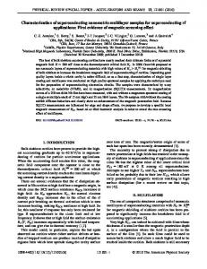
where � and � refer to the classical spherical coordinates (in the case of a counterpropagating scheme � ¼ � ffi and qffiffiffiffiffiffiffiffiffiffiffiffiffiffiffiffiffiffiffiffiffiffiffiffiffiffiffiffiffiffiffiffiffiffiffiffi � ¼ 0) and where u ¼ ð� ¼ 1 þ u2x þ u2y þ u2z ; ux ; uy ; uz Þ is the electron 4-velocity and � its relativistic factor. From there, one can generate a random normal distribution of particles with velocities ux , uy and relativistic factor � and standard deviations �ux ¼ j x =�x , �uy ¼ j y =�y , and �� , respectively. The quantities and � refer to the electron beam normalized emittance and spot size and j to the jitter; j ¼ 1 means that there is no jitter, j ¼ 2 means that the electron beam angular spread is multiplied by two for a given spot size. Figure 1 gives an example of a normalized spectrum obtained with this code. 2. Dose To calculate spectral distribution yielded by the interaction, one has to take into account several other parameters.
(2)
(3)
The most useful expression to describe the source is typically the local differential brightness, which can be derived from the local number of photons scattered per unit time and volume [18]: d� d3 ne d3 n� u k d12 N �ðq � q ; Þ ¼ c d� d3 u d3 k �k d4 xd�dqd3 ud3 k (4) where d3 ne =d3 u and d3 n� =d3 k represent the electron beam phase space density and laser pulse momentum space density. We start with the differential scattering cross section d�=d� described by the Lorentz-boosted Klein-Nishina formula, as derived by Bhatt et al. [19], in which we only use the spin-independent component:
070704-2
CHARACTERIZATION AND APPLICATIONS OF A . . .
Normalized Spectrum
1.0
Phys. Rev. ST Accel. Beams 13, 070704 (2010) In the case of an uncorrelated incident photon phase space, corresponding to the Fourier transform limit, the phase space density takes the form of a product,
0.8
d3 n� ¼ n� ðx Þ~ n� ðk Þ; d3 k
0.6
(8)
the number of photons scattered per unit wave number and solid angle is then given by Z1 ZZZ d� d2 N ¼ �ðq � qc Þ~ n� ½rð�Þ; ��cdt n� ðk Þ d�dq d� �1
0.4
R3
� 3 d k: � �k
0.2
(9)
In our analysis, we consider the case of a plane wave in the Fourier domain:
0.0 0.15 0.20 0.25 0.30 0.35 0.40 0.45 0.50
kx ¼ ky ¼ 0;
Photon Energy MeV FIG. 1. (Color) Example of a spectrum simulated with MATHEMATICA, using 100 000 particles and 100 bins for an electron beam energy of 116 MeV and a laser wavelength of 532 nm (energy 2.33 eV). The other parameters are j ¼ 2, x ¼ 5 mm mrad, y ¼ 6 mm mrad, �x ¼ 35 m, and �y ¼ 40 m.
� � �2 � � d� 1 q 1 � � ¼ ð �c Þ2 þ �1 d� 2 � 2 � � � �� ð u Þð� v Þ ð v Þð� u Þ 2 þ 2 � � þ ; ��c ��c (5) where is the fine structure constant, ¼ ð0; 1; 0; 0Þ corresponds to a linearly polarized incident radiation, and � is the scattered 4-polarization. v ¼ u þ �c ðk � q Þ is the 4-velocity after the scattering event. In the case of a single electron following a trajectory rð�Þ, where � is its proper time, the phase space density is given by a product of Dirac delta distributions: d3 ne ¼ �½x � rð�Þ��½u � uð�Þ� d3 u � � drð�Þ ¼ �½x � rð�Þ�� u � ; cd�
kz ¼ k;
n~� ¼
0 2 exp½�ðk�k Þ� pffiffiffiffi �k : ��k (10)
The integral over k is easily performed by using the fact that �½fðxÞ� ¼
X �ðx � xn Þ jf0 ðxn Þj
;
(11)
where xn represents the poles of the function f. Applying this rule to our case, we first look for the poles kp of qc by solving for qc ðkÞ ¼ 0, and using the above in (9), we find 2 2� � 1 d� � e�ðk�k0 Þ =�k d2 N ¼ pffiffiffiffi ��k d� �k j@k qc ðkÞj k¼kp d�dq Z1 � n� ½rð�Þ; ��cdt: (12) �1
For a Gaussian laser pulse, the incident photon density can be modeled analytically within the paraxial approximation, and in the case of a cylindrical focus: N 1 n� ðx; tÞ ¼ pffiffiffiffiffiffiffiffiffi � 2 �=2w20 c�t3 1 þ ðz=z0 Þ � � � � t � z=c 2 r2 � exp �2 �2 2 ; �t w0 ½1 þ ðz=z0 Þ2 �
(6)
(13)
and thus, after integration over all the electron phase space, the integrated brightness (over the whole surface of the source) reads
where N� is the total number of photons in the laser pulse, �t the pulse duration, w0 the 1=e2 focal radius, and z0 ¼ �w20 =�0 is the Rayleigh range. To evaluate the integral in (12), we replace the spatial coordinates by the ballistic electron trajectory: uy u yðtÞ ¼ y0 þ ct; xðtÞ ¼ x0 þ x ct; � � (14) uz zðtÞ ¼ z0 þ ct; r2 ðtÞ ¼ x2 ðtÞ þ y2 ðtÞ; �
ZZZ d� d3 N d3 n ¼ �ðq � qc Þ 3 � ½rð�Þ; �� cdtd�dq d� dk R3
�
u ð�Þ k 3 d k: �ð�Þ k
(7)
070704-3
F. ALBERT et al.
Phys. Rev. ST Accel. Beams 13, 070704 (2010) Z1 N 1 Ni ¼ �ð1 þ �0 Þ pffiffiffiffiffiffiffiffiffi � 2 2 �=2w0 �t3 �1 1 þ z� � � � � r�2 z 2 � exp �2 0 ðt� � z�Þ2 � 2 dt�; c�t 1 þ z�2
where we can divide x, y, and r by w0 and z and ct by z0 to � y, � z�, r�, and t�. One finally obtain the normalized quantities x, obtains the expression 2 2� � d2 N 1 d� � e�ðk�k0 Þ =�k N� ¼ pffiffiffiffi pffiffiffiffiffiffiffiffiffi 2 d�dq ��k d� �k j@k qc ðkÞj k¼kp �=2w0 c�t3 Z1 1 � 2 �1 1 þ z� � � � � r�2 z 2 � exp �2 0 ðt� � z�Þ2 � 2 dt�: (15) c�t 1 þ z�2
(18)
We finally note that when evaluating (15) it is sufficient to calculate the integral within an interval of �10�t as we assume a Gaussian temporal pulse profile.
where normalized quantities have been used again. To evaluate the integral in (18), we can use again the electron’s ballistic trajectories, as defined in (14). The total dose is then simply obtained by summing over all the macroparticles, and by taking into account the ratio Ne =n between the total number of electrons in the beam and macroparticles in the code. By using this model, we obtain an integrated (over all solid angles) dose of N ¼ 1:32 � 105 photons, for the laser and electron beam parameters summarized in Table I.
3. Integrated dose
III. EXPERIMENTAL METHODS
Calculating the total integrated number of �-ray photons is somewhat simpler. As derived in Ref. [18], the temporal behavior of the �-ray pulse can be described in Cartesian coordinates:
A. Setup overview
d3 N ¼ �ð1 þ �0 Þn� ðr; z; tÞne ðr; z; tÞ; 2�rdrdzcdt
(16)
where ne ðr; z; tÞ is the incident electron beam density and � ¼ 8�r20 =3 is the Compton-scattering cross section. To evaluate the dose yielded by only one macroparticle along its trajectory (re , ze ), one can replace ne ðr; z; tÞ by �ðr ¼ re ; z ¼ ze ; tÞ to end with d3 N i ¼ �ð1 þ �0 Þn� ðr; z; tÞ�ðr ¼ re ; z ¼ ze ; tÞ cdt ¼ �ð1 þ �0 Þn� ðr ¼ re ; z ¼ ze ; tÞ:
The experiments have been performed at the LLNL 100 MeV linac facility, which is located in a well shielded environment, 10 meters below ground, where previous Compton scattering experiments have been performed [20–22]. An overview of the experimental facility is presented in Fig. 2. There were three main caves in which the experiments were made: the outer-detector cave, where the interaction laser system (ILS) was located; the accelerator cave, containing the photocathode and the photoinjector drive laser (PDL), the linac, and the interaction point; and
(17)
In other words, TABLE I. Laser and electron beam parameters used for the integrated dose calculation. 20% compressed means that only 20% of the total laser energy is compressed within the duration of the pulse. Parameter Laser pulse duration Laser wavelength Laser spot size Laser energy Electron energy Electron beam spot size Electron bunch length Electron beam charge Normalized emittance jitter factor
Specification 20 ps (FWHM) 532 nm 34 m (rms), 20% energy in spot 150 mJ, 20% compressed 116 MeV 40 m (rms) 20 ps (FWHM) 0.5 nC 6 mm mrad 2
FIG. 2. (Color) Overview of the experimental facility with the outer-detector (laser) cave, the accelerator cave, and the 0� cave.
070704-4
CHARACTERIZATION AND APPLICATIONS OF A . . .
Phys. Rev. ST Accel. Beams 13, 070704 (2010)
finally the 0� cave, located 20 meters away from the interaction point, on the other side of a thick concrete wall where the �-ray diagnostics, including germanium detectors, were set up. At first light, the � rays were detected on-axis by an intensified CCD mounted on a translation stage. Once the �-ray beam profile was seen on the camera, we translated a 6 mm diameter aperture lead collimator (located 3 meters away from the interaction point) in the beam, and then the camera out, to allow the � rays to propagate in air to the 0� cave. In the 0� cave, the � rays were first detected by a large plastic paddle-shaped scintillator coupled to a 1.3 kV biased photomultiplier. Once � rays correlated to the electron/laser interaction were seen on this detector, spectral measurements using the germanium detectors could be performed. For clarity and comprehension, Sec. III B gives a short description of the three main parts of the setup used to produce � rays: the laser system, the linac, and the interaction region. For a more exhaustive description of the full system, we refer the reader to Gibson et al. [23], and references therein. Then Sec. III C describes the experimental methods used to characterize the beam.
The laser beam is focused to 34 m (rms) and the electron beam is focused using a set of quadrupole magnets with fields of up to 15 T=m. At the focal point, spatial and temporal overlap of the two beams is performed by using an optically polished nickel cube mounted on a three-axis translation stage, with faces that are vertically oriented perpendicular to the beam line, and horizontally oriented at 45� with respect to the beam line. When the electron beam hits the cube, it produces optical transition radiation , and the laser beam is also reflected from the surface. Hence, the position of the two beams at the focal point can be imaged by a CCD camera on one side of the cube for the spatial overlap and by a 100 m slit streak camera providing a 2 ps resolution on the other side for the temporal overlap.
B. -ray light source system The ILS delivers 750 mJ of energy in 16 ps, 0.2 nm bandwidth pulses at 10 Hz. It uses chirped pulse amplification (CPA) [24] in a flashlamp pumped commercial Nd: YAG bulk amplifier fed by a laser oscillator. The key enabling technology is the use of a novel hyperdispersion compressor matched to a chirped fiber Bragg grating stretcher in the front end. The beam after the compressor, initially at 1064 nm, can be frequency doubled or tripled using large aperture deuterated potassium phosphate (DKDP) crystals. For the work here, the 1064 nm pulse of the ILS is frequency doubled using a DKDP crystal, which yields 146 mJ of 532 nm light. The accelerator that provides the electrons starts with a 1.6 cell photocathode gun with a sputtered Mg cathode. This gun is driven by the PDL which shares the oscillator with the ILS to ensure synchronization and provides a 30 J 15-ps flattop spatial and temporal profile at 263.25 nm. This gun produces a charge of 800 pC during normal operation that is then accelerated in five 2.5 m SLAC-type s-band traveling wave sections. The normalized emittance at the end of the beam line is 5–6 mm mrad and it has been measured at low energy using a pepper-pot mask and at high energy with the quadrupole scan technique. After colliding with the laser pulse, the electrons are swept off axis by a 20� dipole magnet to separate the electron bunch from the � rays and to measure the energy spectra of the electron pulses. As it is the configuration that provides the brightest output (all the electrons from the bunch are illuminated by the ILS), the laser and electron beams collide at 180�.
C. Methods and diagnostics for -ray beam characterization 1. Spatial and temporal measurements The � rays are detected on axis by a system which is comprised of a 16 bit intensified charge coupled device (ICCD) Andor camera and a 3:1 optical fiber reducer coupled to the camera. The ICCD chip is an array of 1024 � 1024 13 m size pixels coupled to a 1:1 optical fiber bundle, which, with the reducer demagnification, provides a 4 � 4 cm2 detection surface. The fiber reducer is coupled to a 140 m cesium iodine scintillator doped with thallium [CsI(Tl)], which isotropically converts the � rays into visible green light at a rate of 54 photons=keV. The scintillator is protected with a 0.5 mm thick beryllium (Be) window to block any laser light remaining and to cut detected noise from low energy x rays scattering in the accelerator cave. The system was calibrated by using a 137 Cs radioisotope source delivering 2:85 � 105 photons=s at 662 keV. The measurements indicate 70 counts=photon at this energy (one gamma-ray photon yields 70 counts on the CCD). From that point, the number of counts per �-ray photon produced by the detection system can be extrapolated by using the �-ray absorption curve in CsI(Tl), which can be found in the NIST X-COM database [25]:
CðEÞ ¼
E 1 � e�� ðEÞ� CðE0 Þ ; E0 1 � e�� ðE0 Þ�
(19)
where � ¼ 140 m is the scintillator thickness, E0 ¼ 662 keV is the energy of the calibration source, r ¼ 4:51 g=cm3 is the density of CsI(Tl), and ðEÞ is the mass absorption coefficient, in square centimeters per gram. Because we made the calibration at a different energy (662 keV) than that of our source (478 keV), Eq. (19) basically takes into account the fact that the detector response is not constant with energy.
070704-5
F. ALBERT et al.
Phys. Rev. ST Accel. Beams 13, 070704 (2010)
2. Spectral measurements Several techniques are currently available to measure xray spectra, including Bragg diffraction crystals, filters relying on x-ray attenuation in materials, and photoncounting methods with scintillators or x-ray diodes. As the lattice spacing for a diffraction crystal has to be on the order of the wavelength of the diffracted radiation to obtain a good resolution and efficiency, no crystal allows us to use this technique at energies of a few 100 keV and above. Using filters in our case is impractical because high Z and very thick materials would be needed, and the resolution of the measurement would be poor. For our spectral experiments we decided to use a detector operating in a statistical single photon-counting mode. In the present geometry, the �-ray detector would have to be directly in the high-energy bremsstrahlung produced by the dark current of the linac if we want to measure the spectrum on axis. This yields background levels that are incompatible with single photon counting. To avoid this problem, we chose a geometry where the � rays are detected by a high purity germanium detector (HPGe) at an angle � ¼ 48� with respect to the main beam axis, after being scattered off a 1=8 inch thick aluminum (Al) plate located 20 meters away from the interaction point, in a room where the system is shielded by concrete walls. With this layout, as depicted on Fig. 3, the scattered � rays of energy E� are related to the incident � rays of energy E� by the Compton-scattering relation: E0� ¼
E� 1þ
E� E0
ð1 � cos�Þ
;
of the Al plate was adjusted so that a count rate of 0:2 photon=shot was observed on the HPGe, which we judged as the best tradeoff between pileup and efficiency. The detector is made of a high purity germanium crystal which is 8 cm long and 6 cm in diameter. The resolution, measured with a 137 Cs radioisotope source, was found to be 2.8 keV at 662 keV (0.4%). The detector head is placed 150 cm away from the Al plate, which corresponds to an angle of 2.3� subtended by the crystal. With a scattering angle of 48 degrees and a central energy of 478 keV (scattered energy 365 keV), this means an uncertainty of 13 keV on the spectrum measurement (relative uncertainty of 3.5%). The resolution of our spectrum is thus limited by the geometry of our detection system. The output signal of the detector, biased at þ4000 Volts, is shaped to a pulse with an amplitude ranging from 1 to 10 Volts and with a full width half maximum (FWHM) of several s. This pulse is then sent to a 8192-channel analog to digital converter (ADC) which retrieves the spectrum. The ADC was synchronized to the rf power of the linac with a 8 s gate, to ensure that only photon events related to the linac and Compton scattered � rays at 10 Hz where recorded. This was necessary because of the natural activation present in the room, at a rate of several kHz, which makes the detection of the Compton scattered �-rays spectrum impossible. The settings of the shaper and ADC allowed us to measure spectra in the 10 keV–1.6 MeV range with a dispersion of 0:2 keV=channel.
(20)
where E0 ¼ 0:511 MeV is the electron rest energy. This method has two advantages: the detector is placed far from the on-axis bremsstrahlung background and the Al plate preferentially scatters the lower energy � rays. For example, 7% of 500 keV radiation is attenuated by the plate while only 2.5% of 5 MeV � rays are. The thickness
IV. EXPERIMENTAL RESULTS This section presents a complete characterization of the source mainly when the electron beam is tuned at 116 MeV and the laser at 532 nm (second harmonic generation of 1064 nm infrared light produced by the ILS). We have also produced � rays with laser light from first (1064 nm) and third (355 nm) harmonic generation, and the results are presented for completeness, although no exhaustive characterization has been made at these energies. On axis, if we have 116 MeV electrons and 532 nm laser light, the scattered energy is 478 keV, according to (1). Our motivation for selecting this energy was to detect nuclear resonance fluorescence (NRF) in 7 Li, which has a strong line at 478 keV. At this energy, the following features of the source have been studied: �-ray beam profile and dose, source size, dose as a function of delay between the laser and the electron beam, on and off-axis spectrum, and tunability with the electron beam energy. A. Spatial and temporal properties of the source 1. Beam profile and dose
FIG. 3. (Color) Layout of the detection system. The � rays are detected by a HPGe detector after being Compton scattered off an Al plate at 48 degrees.
The spatial beam profile was measured with the Andor camera using 15 s integration time (150 shots at 10 Hz) to obtain good statistics. Figure 4 shows a typical �-ray image recorded with those conditions 2 m away from the
070704-6
CHARACTERIZATION AND APPLICATIONS OF A . . .
Phys. Rev. ST Accel. Beams 13, 070704 (2010)
Energy Density (arb. units)
1.0
0.8
0.6
0.4
0.2
0.0 − 0.015 − 0.010 − 0.005 0.000 0.005 0.010 0.015 Angle Along x−Axis (Rad) 0.015
Angle Along y−Axis (Rad)
0.010 0.005 0.000 − 0.005 − 0.010 − 0.015 0.0
0.2 0.4 0.6 0.8 1.0 Energy Density (arb. units)
1.2
FIG. 4. (Color) False color image of the � rays recorded by the ICCD over 15 s of integration at 10 Hz and 2 m away from the interaction region. On the bottom and left of the image, the angular energy distribution are displayed for the horizontal (x) and vertical (y) axis, respectively. The solid curves represent the Gaussian fit of the experimental data points (dots).
interaction region. The divergence is lower along the horizontal direction due to polarization effects [26]. The full width half maximum (FWHM) of the beam is 6.0 mrad and 10.4 mrad along the horizontal (x) and vertical (y) axis, respectively. By integrating the total counts from the beam profile in Fig. 4, one obtains a total number of 1:6 � 105 photons=shot. 2. �-ray intensity as a function of delay between laser and electron beams When the laser and electron beams are collinear, varying the delay is equivalent to a change in the laser spot size from its minimum waist w0 and photon density at the interaction point. Thus, the �-ray intensity as a function
of the delay between the two beams varies as a Lorentzian 1=½1 þ ðz=z0 Þ2 �, where z0 ¼ �w20 =�0 is the Rayleigh length. Since the beta function of the electron beam focusing line is longer than the Rayleigh length in our geometry, the �-ray intensity variation is dominated by the change in the laser spot size. We have used an optical delay line to vary the timing between the laser pulse and the electron bunch, which allowed us to measure the �-ray intensity change, averaged over 25 shots, displayed on Fig. 5. The experimental curve can be fitted by a Lorentzian of width �t ¼ 25 ps, which corresponds to a Rayleigh length z0 ¼ c�t ¼ 7:5 mm. The focal spot inferred from this measurement is 29 m (FWHM) at �0 ¼ 532 nm. This value is 2.5 times smaller than the actual FWHM focal spot size (w0 ¼ 75 m), indicating a nondiffraction limited laser opera-
070704-7
F. ALBERT et al.
Phys. Rev. ST Accel. Beams 13, 070704 (2010)
Normalized X ray dose
3000 2500 2000 1500 1000 500 40
20
0
20
40
60
80
100
Delay ps
FIG. 5. (Color) Experimentally measured variation of the �-ray intensity as a function of the delay t between the laser and the �-ray beams (dots) and Lorentzian fit 1=½1 þ ðt=�tÞ2 �, where �t ¼ 25 ps (dashed curve). The error bars are the standard deviation of the intensity averaged over 25 shots.
tion. On Fig. 5 one can observe a ripple for delays larger than 40 ps that deviates from the theoretical Lorentzian shape. It is explained by the fact that the laser pulse was not optimally compressed. Indeed, we recorded autocorrelation traces of the compressed pulse, which indicated that only �20% of the total energy (at 1064 nm) was within 16 ps and that the rest was contained in wings on each side of the compressed pulse. B. Spectral measurements 1. On-axis spectra In Fig. 6, the spectrum of on-axis photons is shown. To faithfully measure the on-axis spectrum, we have used a 6 mm diameter lead collimator to aperture the beam, placed 3 meters away from the interaction point. The collimator was aligned to the center of the spatial image, as shown in the inset of Fig. 6. The spectrum displayed in
Normalized Spectrum
1.0 0.8 0.6 0.4 0.2 0.0 0
200
400
E
600
keV
FIG. 6. (Color) On-axis spectrum recorded after scattering off the Al plate and corresponding Monte Carlo simulation. The images correspond to the full beam and the signal transmitted through the collimator, respectively.
Fig. 6 corresponds to 5 keV bins and to 6.5 hours of data recorded at 10 Hz. The measured spectrum is compared with the simulated pulse height spectrum expected for single-photon counting. As can be seen in Fig. 6, the spectrum has several distinctive features. The tail after 400 keV is mainly due to the high-energy bremsstrahlung and to pileup (multiplephoton events) in the detector. The main peak has a maximum for 365 keV, which corresponds to an incident energy of 478 keV. The FWHM of this peak is 55 keV (within limitation of 5 keV bins), which corresponds to a relative bandwidth of 15%. By differentiating (20), it corresponds to source (at the aluminum plate) bandwidth of 12%. The narrower energy spectra (on the order of 1% reported in Ref. [18]) have been computed with different parameters that were not the measured experimental parameters in our case. In particular, the bandwidth of the gamma-ray spectrum increases as the square of the normalized emittance, which is the most critical point for the design of a narrow band Compton-scattering source. The energy spread and jitter of the laser are negligible, while those of the electron beam are 0.2% and j ¼ 2, respectively. This means that the broadening effect on the gamma rays is, using Eq. (1), 0.4% from the electron beam energy spread. It is much smaller than the broadening effect (4.5%) due to the electron beam divergence =�r, where r is the electron beam radius. The fact that we obtained a bandwidth of 12% can also be explained by nonlinear broadening effects and by the electron beam position and angular jitter, since we are not showing a single shot but an average (over several hours) spectrum in Fig. 6. At energies lower than 250 keV, a broad continuum can be seen, on which two other peaks (respectively located around 80 and 110 keV) are superposed. Those are not physical features of the source itself but are the result of several interaction processes, which can be very well tracked and reproduced by Monte Carlo simulations. For modeling we used the MCNP5 code [27], with modifications to include Compton scattering of linearly polarized photons [28]. The �-ray source spectrum was calculated using the MATHEMATICA script described in Sec. II, and used by MCNP5 to sample the energy of each source photon in the incident pencil beam (5 cm diameter). The polarization was assumed to be 100% in the horizontal plane (including the beam axis and HPGe detector). All the major components of the experimental setup, such as walls, air, and lead shielding were implemented in the MCNP5 geometry description. Figure 6 shows the simulated pulse height spectrum expected for single-photon counting. The continuum below 250 keV is due to incomplete energy absorption (elastic Compton scattering) in the detector itself. The broad peak at 110 keV arises from double Compton scattering off the Al plate and adjacent wall, followed by photoabsorption in the Ge detector. Since the detector is shielded with lead, the first peak is due to x rays
070704-8
CHARACTERIZATION AND APPLICATIONS OF A . . .
Phys. Rev. ST Accel. Beams 13, 070704 (2010)
coming from the lead K and K� lines, respectively, at 72.8, 75, 84.9, and 87.3 keV. The 5 keV binning applied to the spectrum does not allow us to distinguish those lines.
2.5 mrad off-axis measurement in the lower part of the beam, as shown in Fig. 7. As expected, for both lobes the spectrum is broader than on-axis, with a peak at �250 keV for the upper lobe and a peak at �290 keV for the lower lobe as seen on the plots resulting from the Monte Carlo simulation with MCNP5. The parameters of the simulation are the same as for the on-axis spectrum calculation except for the angle of observation that has been changed according to the upper and lower part of the beam.
2. Off-axis spectra: energy-angle correlation The energies of � rays produced by Compton scattering vary within the cone of radiation. According to (1), the highest �-ray energy 4�2 EL is on-axis and the off-axis �-ray energies should be lower. To verify this characteristic property of Compton scattering we have measured the spectrum off-axis, at two different positions, for an electron beam energy of 125 MeV and a laser wavelength of 532 nm. To do so, we have used the same 6 mm lead aperture as for the on-axis measurement, and to alter the direction of the �-ray beam, the incident electron beam was deflected with two small steering magnets, so that the position of the electrons at the interaction point was fixed, while the beam angle could be varied by several milliradians. It was not possible to move the collimator instead as it is precisely pointing toward the shielded room where the detectors are. Our measurements correspond to a 3 mrad off-axis measurement in the upper part of the beam and to a
3. Energy scaling with the electron beam energy On axis, the Compton scattered �-ray energy theoretically scales with 4�2 for a given laser photon energy (if we neglect the recoil), which we verified by tuning the electron beam to four different energies: 116, 101, 85, and 68 MeV, and by measuring the spectrum for each case. Identical alignment of the collimator with the center of the beam has been maintained throughout the measurement. The four spectra are displayed in the top part of Fig. 8, where each data set corresponds to 1 h of acquisition at 10 Hz and in a single photon-counting mode (rate of 20%). The 116 MeV data correspond to 6.5 hours of acquisition and has been
300
Counts/(5 keV bin hour)
Counts / 5 keV bin
2.0
1.5
1.0
0.5
250 200 150 100 50 0
0.0
100
200
300
100
400
400
500
500
X−ray energy (keV)
1.4 1.2
Counts / 5 keV bin
300
X−ray Energy (keV)
Energy keV
1.0 0.8 0.6 0.4 0.2 0.0
200
400 300 200 100 0 0
0
100
200
300
400
20
40
60
80
100
120
Electron Energy MeV
Energy keV
FIG. 7. (Color) Off-axis spectra measured (dots) for the upper lobe (3 mrad away from the center) and the lower lobe (2.5 mrad away from the center), with the corresponding Monte Carlo simulations (dashed curves).
FIG. 8. (Color) Top: Experimentally measured on-axis spectra for electron beam energies of 68 MeV (dot-dashed line), 85 MeV (dotted line), 101 MeV (dashed line), and 116 MeV (solid line). Bottom: experimentally measured peak �-ray energy points versus � and theoretical peak �-ray energy Ex ¼ 4�2 EL .
070704-9
F. ALBERT et al.
Phys. Rev. ST Accel. Beams 13, 070704 (2010)
normalized to be within the same amplitude as the other plots. From this measurement, the incident peak �-ray energy on the Al plate can be retrieved by using (20). The bottom part of Fig. 8 displays the incident peak �-ray energy (inferred from the experimental data) versus the electron relativistic factor �. On top of the data points is plotted the theoretical expected �-ray energy 4�2 EL , where EL ¼ 2:33 eV is the laser energy. This shows good agreement and validates the 4�2 signature scaling law of laser-based Compton scattering for our source.
C. Summary: On-axis peak brilliance
Brightness Nx s mm2 mrad2 0.1
Counts/(100 keV bin hour)
The linac itself is a source of high-energy � rays because it is well known that the electromagnetic field in a high gradient rf structure can cause electron emission from the copper walls of the accelerating sections. Those electrons can then be accelerated by the fields and interact with metal present in the linac, which potentially yields high-energy � rays on axis. The dark current can reduce the signal to noise ratio for the Compton scattered � rays. To measure this background, we placed one HPGe directly in the incident beam. During this measurement, only the rf power of the linac was enabled while all the lasers (ILS and PDL) were turned off. In addition, to avoid saturation on the detector, we placed 5 inches of lead in the beam path to reduce the count rate to 0:2=pulse. Since low energy x rays are highly attenuated by the lead absorber, only bremsstrahlung arising from the dark current was measured. The resulting spectrum is presented in Fig. 9, on which the 0.511 MeV line from electron-positron annihilation pairs can well be seen. The incident number of �-ray photons on the detector can be simply retrieved by taking into account the attenuation through 5 inches of lead (NIST-XCom database) and the efficiency of the detector (50%). At 1 MeV, one finds 1:1 photons=0:1%BW=shot from bremsstrahlung.
200
150
511 keV Line
100
50
0 0
2
bw
4. High-energy bremsstrahlung
With the experimental results obtained throughout the experiments, one can compute the on-axis peak brilliance of the source. The only parameter that has not been directly measured during this experimental campaign is the Compton gamma-ray source size. However, it can be inferred from the overlap of the electron beam and laser beam focal spots, which have been measured at 40 m (rms) and 34 m (rms), respectively. With a spectral bandwidth of 12% at 478 keV, a pulse duration of 16 ps (FWHM, inferred from the laser and electron beam durations), a dose of 1:6 � 105 photons=shot, and a divergence of 10:4 � 6 mrad2 (FWHM), one obtains an on-axis peak brilliance of 1:5 � 1015 photons=mm2 =mrad2 =s=0:1% bandwidth, which is roughly the brilliance of the APS synchrotron at this energy, currently the brightest synchrotron in the United States [5]. However, since the main goal of this experiment was the proof of principle demonstration of NRF, neither the laser nor the electron beam were fully optimized. However, by using the code described in this paper and that has been benchmarked against our experimental results, we can predict a peak brilliance on the order of 1 � 1021 photons=mm2 =mrad2 =s=0:1% bandwidth at 478 keV by using state of the art parameters for the electron (1 nC, 1 mm mrad) and laser (1 J) beams, as shown in Fig. 10, with detailed parameters specified in Table II. This is 6 orders of magnitude higher than the brightness we currently achieved. Several reasons can explain why we did not reach state of the art parameters in the present source: The linac we used is 40 years old, and the radiofrequency (rf) power is asymmetrically fed to the sections,
4
6
8
6 1021 5 1021 4 1021 3 1021 2 1021 1 1021 0 0.46
0.47
0.48
0.49
0.50
Photon Energy MeV
gamma−ray energy (MeV)
FIG. 9. (Color) High-energy bremsstrahlung arising from the linac dark current measured between 0 and 8 MeV (100 keV bins) and behind 5 inches of lead.
FIG. 10. (Color) On-axis spectrum calculated with a 1 nC, 1 mm mrad emittance and 9 m electron beam spot size (rms) and a 1 J, 9 m rms size laser spot and no jitter.
070704-10
CHARACTERIZATION AND APPLICATIONS OF A . . .
Phys. Rev. ST Accel. Beams 13, 070704 (2010)
TABLE II. State of the art laser and electron beam parameters used for the brightness calculation. Specification
Laser pulse duration Laser wavelength Laser spot size Laser energy Electron energy Electron beam spot size Electron bunch length Electron beam charge Normalized emittance Jitter factor
10 ps (FWHM) 532 nm 9 m (rms), 100% energy in spot 1 J, 100% compressed 116 MeV 9 m (rms) 10 ps (FWHM) 1 nC 1 mm mrad 1
which induces emittance growth as the electrons are accelerated. The laser compression was not optimized, and therefore, all the energy was not contained in the compressed pulse. We used a chirped fiber Bragg grating stretcher, which is very sensitive to temperature variations, and a bulk grating compressor. Because the bandwidths involved here are extremely narrow for chirped pulse amplification, the compressor path length had to be very long (30 m). We estimate the infrared short pulse to contain only 20% of the total energy. Because of the above reason, the nonlinear conversion from infrared to green light was relatively poor. Those technological bottlenecks are being addressed for the design of the next monoenergetic gamma-ray (MEGa-ray) source at LLNL. The focal laser sport size, measured to be 34 m (rms), did not contain all the energy as well, as shown on beam profile measurements. We had at most 20% of the total laser energy as well. V. APPLICATION: DETECTION OF NUCLEAR RESONANCE FLUORESCENCE IN 7 LI A. NRF detection setup In addition to measuring the properties of the source, we have used it to detect the NRF line of 7 Li at 478 keV. For this, we used a 8-cm diameter plastic bottle containing 225 g of LiH with a density of 0:36 g=cm3 . The sample was located in the shielded 0� cave, about 20 meters away from the source which is still collimated by the 6-mm lead aperture. When the beam interacts with the lithium, its diameter is on the order of 4 cm. The NRF scattered photons from the 7 Li are detected by a second HPGe, similar in size, resolution, and efficiency to the one used for the spectral measurements. As depicted in Fig. 11, the detector is placed at 90� with respect to the incident beam axis, 15 cm away from the center of the beam. As only 7% of the incident � rays are attenuated by the Al plate, we have kept the spectral diagnostic in order to verify the proper tuning of the beam throughout the measurement.
Incident γ rays Compton scattered γ rays 10%
HPGe Detector 2 NRF Detection HPGe Detector 1 Spectum Measurement
Concrete walls Separation from LINAC
FIG. 11. (Color) NRF detection setup.
With the �-ray production described above at 478 keV, NRF photons were expected to be scattered isotropically at a rate of 16 photons=hour. The HPGe detector was positioned in the x-ray polarization plane to maximize the NRF signal from the M1 transition in 7 Li [29]. A scattering angle of 90� was chosen in order to minimize the amount of Compton scatter background from the LiH target [30]. A 1 cm thick Pb absorber in front of the HPGe detector reduced the count rate to 10%. It also serves as a demonstration that detecting low-Z and low-density material behind high-Z, high-density material is feasible with this process. Indirect detection methods have also been successfully employed with this source [31] B. NRF results NRF data have been acquired for 7.5 hours at a 10 Hz repetition rate and the full spectrum obtained on the detector between 0 and 1.6 MeV is displayed in Fig. 12 on a logarithmic scale. Besides the 478 keV NRF line from 7 Li, several distinguishable features can be observed on this plot. The continuum centered around 250 keV corresponds to Compton scattering of the 478 keV radiation off the LiH sample at an angle of 90�. As in the source spectrum, the peaks corresponding to the lead fluorescence around 80 keV are present. The line at 511 keV results from the
10.00 Pb Fluorescence 5.00
Signal (arb. unit)
Parameter
Al plate
Transmitted γ rays 90% LiH sample NRF 7Li at 478 keV Θ = 48°
070704-11
Continuum
1.00 0.50
511 keV
NRF
Co Lines
0.10 0.05 0.01
0
200
400
600
800
1000
Energy (keV)
FIG. 12. NRF spectrum and features.
1200
1400
F. ALBERT et al.
Phys. Rev. ST Accel. Beams 13, 070704 (2010)
Counts/keV Bin (arb. unit)
ACKNOWLEDGMENTS 100
This work performed under the auspices of the U.S. Department of Energy by Lawrence Livermore National Laboratory under Contract No. DE-AC52-07NA27344. The authors wish to thank Gerry Anderson for the electron beam operations and detectors shielding, and Shawn Betts for laser operations.
80 60 40 20 0 460
480
500
520
Energy (keV)
FIG. 13. (Color) NRF scattered spectrum between 460 and 540 keV, showing the NRF line with a 6� confidence level and the 511 keV line.
eþ � e� annihilation pairs created by the high-energy bremsstrahlung from the linac (this line remains present when we block the ILS). The lines at 1.17 and 1.33 MeV arise from 60 Co activation naturally present in the cave walls. A closer look at the scattered spectrum between 460 and 540 keV (Fig. 13), showing the NRF line and the 511 keV line, indicates a detection confidence level of 6�, which means that statistically (assuming a normal distribution with standard deviation �), we are above the background so that the confidence of our measurement is superior to 99.99%. Because the theoretical width of the NRF line from 7 Li (a few eV) is much lower than the measured resolution of the germanium detector (2.8 keV), it is not possible to estimate the experimental width of the line. VI. CONCLUSION AND OUTLOOK In conclusion, we have demonstrated and characterized Compton scattering from a novel high-brightness �-ray source. This source has been exhaustively studied by a series of different diagnostics, allowing us to measure spectral (12% bandwidth at 478 keV) and spatial data (low divergence), as well as characteristic signatures of the Compton-scattering mechanism (4�2 scaling and energy-angle correlation). The key parameter of this source is its peak brilliance, 1:5 � 1015 photons=mm2 = mrad2 =s=0:1% bandwidth at MeV-range energies. As it scales with the square of the electron beam relativistic factor divided by its normalized emittance, it will be enhanced at higher �-ray energies by pursuing the development of new technologies associated with this source. High acceleration gradient x-band linac systems, robust and high-average power fiber laser systems are all part of the design of a new MEGa-ray precision machine currently developed at LLNL. In this paper, we have demonstrated, by detecting nuclear resonance fluorescence from 7 Li at 478 keV, that this new class of Compton-scattering sources will have tremendous applications in nuclear photoscience.
[1] R. Schoenlein, W. Leemans, A. Chin, P. Volfbeyn, T. Glover, P. Balling, M. Zolotorev, K. Kim, S. Chattopadhyay, and C. Shank, Science 274, 236 (1996). [2] A. Rousse, C. Rischel, and J-C. Gauthier, Rev. Mod. Phys. 73, 17 (2001). [3] F. Zernike, Science 121, 345 (1955). [4] E. Roessl and R. Proksa, Phys. Med. Biol. 52, 4679 (2007). [5] D. Attwood, Soft X-rays and Extreme Ultraviolet Radiation (Cambridge University Press, Cambridge, England, 1999), Chap. 5. [6] http://ssrl.slac.stanford.edu/lcls/. [7] http://www.xfel.eu/. [8] U. Kneissl, H. M. Pitz, and A. Zilges, Prog. Part. Nucl. Phys. 37, 349 (1996). [9] P. Coleman, Positron Beams and Their Applications (World Scientific, Singapore, 2000). [10] H. R. Weller, M. W. Ahmed, H. Gao, W. Tornow, Y. K. Wu, M. Gai, and R. Miskimen, Prog. Part. Nucl. Phys. 62, 257 (2009). [11] V. N. Litvinenko, Nucl. Instrum. Methods Phys. Res., Sect. A 507, 527 (2003). [12] F. V. Hartemann, H. A. Baldis, A. K. Kerman, A. Le Foll, N. C. Luhmann, Jr., and B. Rupp, Phys. Rev. E 64, 016501 (2001). [13] W. P. Leemans, R. V. Schoenlein, P. Volfbeyn, A. H. Chin, T. E. Glover, P. Balling, M. Zolotorev, K-J. Kim, S. Chattopadhyay, and C. V. Shank, IEEE J. Quantum Electron. 33, 1925 (1997). [14] S. K. Ride, E. Esarey, and M. Baine, Phys. Rev. E 52, 5425 (1995). [15] F. V. Hartemann and A. K. Kerman, Phys. Rev. Lett. 76, 624 (1996). [16] E. Esarey, S. K. Ride, and P. Sprangle, Phys. Rev. E 48, 3003 (1993). [17] F. V. Hartemann, High Field Electrodynamics (CRC Press, Boca Raton, FL, 2002). [18] F. V. Hartemann, W. J. Brown, D. J. Gibson, S. G. Anderson, A. M. Tremaine, P. T. Springer, A. J. Wootton, E. P. Hartouni, and C. P. J. Barty, Phys. Rev. ST Accel. Beams 8, 100702 (2005). [19] G. Bhatt, H. Grotch, E. Kazes, and D. A. Owen, Phys. Rev. A 28, 2195 (1983). [20] D. J. Gibson, S. G. Anderson, C. P. J. Barty, S. M. Betts, R. Booth, W. J. Brown, J. K. Crane, R. R. Cross, D. N. Fittinghoff, F. V. Hartemann, J. Kuba, G. P. Lesage, D. R. Slaughter, A. M. Tremaine, A. J. Wooton, E. P. Hartouni, P. T. Springer, and J. B. Rosenzweig, Phys. Plasmas 11, 2857 (2004).
070704-12
CHARACTERIZATION AND APPLICATIONS OF A . . .
Phys. Rev. ST Accel. Beams 13, 070704 (2010)
[21] W. J. Brown, S. G. Anderson, C. P. J. Barty, S. M. Betts, R. Booth, J. K. Crane, R. R. Cross, D. N. Fittinghoff, D. J. Gibson, F. V. Hartemann, E. P. Hartouni, J. Kuba, G. P. Le Sage, D. R. Slaughter, A. M. Tremaine, A. J. Wooton, and P. T. Springer, Phys. Rev. ST Accel. Beams 7, 060702 (2004). [22] F. V. Hartemann, A. M. Tremaine, S. G. Anderson, C. P. J. Barty, S. M. Betts, R. Booth, W. J. Brown, J. K. Crane, R. R. Cross, D. J. Gibson, D. N. Fittinghoff, J. Kuba, G. P. Le Sage, D. R. Slaughter, A. J. Wootton, E. P. Hartouni, P. T. Springer, J. B. Rosenzweig, and A. K. Kerman, Laser Part. Beams 22, 221 (2004). [23] D. J. Gibson et al., preceding article, Phys. Rev. ST Accel. Beams 13, 070703 (2010). [24] D. Strickland and G. Mourou, Opt. Commun. 56, 219 (1985).
[25] http://physics.nist.gov/PhysRefData/Xcom/Text/ XCOM.html. [26] W. J. Brown and F. V. Hartemann, Phys. Rev. ST Accel. Beams 7, 060703 (2004). [27] R. A. Forster et al., Nucl. Instrum. Methods Phys. Res., Sect. B 213, 82 (2004). [28] G. Matt, M. Feroci, M. Rapisarda, and E. Costa, Radiat. Phys. Chem. 48, 403. [29] N. Pietralla et al., Phys. Rev. Lett. 88, 012502 (2001). [30] L. W. Fagg and S. S. Hanna, Rev. Mod. Phys. 31, 711 (1959). [31] F. Albert, S. G. Anderson, G. A. Anderson, S. M. Betts, D. G. Gibson, C. A. Hagmann, J. Hall, M. S. Johnson, M. J. Messerly, V. A. Semenov, M. Y. Shverdin, A. M. Tremaine, F. V. Hartemann, C. W. Siders, D. P. McNabb, and C. P. J. Barty, Opt. Lett. 35, 354 (2010).
070704-13