Keywords: waveform-agile sensors, tracking, clutter, CRLB ... use in agile sensing. .... k bi k]T is the waveform parameter vector and λi k = T + 2tf is the signal ...
Characterization of Waveform Performance in Clutter for Dynamically Configured Sensor Systems Sandeep P. Sira, Antonia Papandreou-Suppappola
Darryl Morrell
Department of Electrical Engineering Arizona State University
Department of Engineering Arizona State University
Keywords: waveform-agile sensors, tracking, clutter, CRLB ABSTRACT In this paper, we consider the problem of dynamic selection of frequency modulated waveforms and their parameters for use in agile sensing. The waveform selection is driven by a tracker that uses probabilistic data association to track a single target in clutter, employing measurements derived from a nonlinear observations model. We present an algorithm that performs the selection so as to minimize the predicted mean square error which is computed using the unscented transform. We compare and analyze the performance of several trapezoidal envelope frequency modulated waveforms with different time-frequency structures using the Cram´erRao lower bound. The simulation results indicate that the dynamic selection of waveforms and their corresponding parameters improves the tracking performance. 1. INTRODUCTION As modern sensors become increasingly more capable, it is possible to consider their dynamic adaptation so that they contribute optimally towards the overall system objective. In the past, tracking algorithms and sensors have been optimized independently [1]. While this improves system capabilities, it does not necessarily yield the best overall performance. The ability to configure waveform-agile sensors to obtain information that best improves the tracker’s current estimate provides a means of optimizing the system as a whole and can yield significantly better results. The dynamic selection of waveforms for target tracking was first considered in [2], where the optimal waveform parameters were derived for tracking one-dimensional target motion using observations that were a linear function of the target state. The measurement model was extended to include clutter and imperfect detection but the linearity in the observations was still assumed in [3]. Other work on waveform optimization for target tracking with similar observations models includes [4, 5]. However, such simple
tracking scenarios do not occur in practice. As a consequence, sub-optimal estimators of the target state have to be considered, thus precluding the determination of optimal waveform designs. In this paper, we consider a nonlinear observations model in the problem of dynamically configuring the waveforms transmitted by two active waveform-agile sensors in the presence of clutter and missed detections. Specifically, we select the phase function and configure the duration and frequency modulation (FM) rate of generalized chirp waveforms. Using these waveforms, the sensors generate range and Doppler measurements to track a target moving in two dimensions. The target tracker is implemented using a particle filter that employs probabilistic data association to deal with the uncertainty in the origin of the measurements due to clutter. The waveforms are configured to minimize the predicted mean squared error (MSE) where the prediction is performed using the Cram´er-Rao lower bound (CRLB) on the measurement errors. We develop an algorithm that performs the waveform configuration and use it to compare the performance of different types of generalized FM chirp waveforms. The layout of the paper is as follows. In Section 2, we describe the waveform structure and the target dynamics model. In Section 3, we describe the measurement model, and in Section 4, the target tracking algorithm is considered. In Section 5, we describe the dynamic waveform selection algorithm and present simulation results in Section 6.
2. TARGET KINEMATICS AND WAVEFORM STRUCTURE We seek to estimate the motion of a target that is free to move in two dimensions. The target state is given by Xk = [xk yk x˙ k y˙ k ]T , where xk and yk correspond to the position, and x˙ k and y˙ k to the velocity, at time k in Cartesian coordinates.
2.1. Target dynamics
6
x 10
The target dynamics are modeled by a linear, constant velocity model given by
14
PFM κ = 2.8
Xk = F Xk−1 + Wk .
12
The process noise is modeled by the uncorrelated Gaussian sequence Wk . The constant matrix F and the process noise covariance Q are given by 1 0 δt 0 0 1 0 δt F = 0 0 1 0 , 0 0 0 1 3 δt δt2 0 0 3 2 δt3 δt2 0 0 3 2 Q = q δt2 (2) , 2 0 δt 0 2 δt 0 0 δt 2
10
where δt is the sampling interval and q is a constant. The target motion is observed by two active sensors, A and B, which measure the range and range-rate of the target. The sensors are waveform-agile as they can change their waveform from pulse to pulse. 2.2. Waveform structure At each sampling instant, each of the sensors transmits a generalized chirp whose complex envelope is given by s˜(t) = a(t) exp (j2πbξ(t/tr )),
|t| < T /2 + tf , (3)
where b is a scalar FM rate parameter, tf ¿ T /2 is a rise/fall time for the trapezoidal envelope a(t), and tr > 0 is a reference time point. We can obtain different FM waveforms with unique time-frequency signatures by varying the phase function ξ(t/tr ) and thus the waveform’s d instantaneous frequency dt ξ(t/tr ). The waveforms considered in this paper are the power FM (PFM), hyperbolic FM (HFM) and the exponential FM (EFM) chirps. The phase function and frequency sweep of each is shown in Table 1 with the reference time tr = 1. The PFM chirp
Waveform
Phase Function ξ(t)
Frequency sweep
PFM
t/Tf + (t + λ/2) /κ
b( T1f + λ)
HFM
ln(t + Tf + λ/2)
b Tf (Tλf +λ)
EFM
κ
exp(−(t + λ/2)/Tf )
− Tλ f
b T1f (e
− 1)
Table 1. FM waveforms used in the configuration scenarios. The parameter Tf and the FM rate b in (3) determine the frequency sweep, and λ is the pulse duration.
Frequency (Hz)
(1)
LFM
8
6
4
EFM
2
HFM 0
0.1
0.2
0.3
0.4
0.5
0.6
0.7
Time (s)
0.8
0.9
1 −4
x 10
Fig. 1. Time-frequency plots of generalized FM chirp waveforms (downsweep - solid lines, upsweep - dotted lines) with duration 100 µs and frequency sweep 14 MHz. is characterized by the power κ. The linear FM (LFM) chirp results when κ = 2. Fig. 1 shows the instantaneous frequencies of these waveforms for a duration of 100 µs and a frequency sweep of 14 MHz. The time varying amplitude in (3) is given by α T tf (t − 2 − tf ), −T /2 − tf ≤ t < −T /2 α, −T /2 ≤ t < T /2 a(t) = α ( T + tf − t), T /2 ≤ t < T /2 + tf , tf 2 where α is an amplitude chosen so that the signal has unit energy. Using a trapezoidal envelope avoids the difficulties associated with the evaluation of the CRLB for rectangular envelopes [6] and provides a clearer comparison of phase function performance than using a Gaussian envelope. With a Gaussian envelope [7], the behavior of the phase function in the tails of the envelope does not significantly affect the waveform’s performance in range and Doppler estimation, since the tails contain a small fraction of the signal energy. 3. MEASUREMENT MODEL The waveform transmitted by sensor i (i = A, B) reflects off the target and is received at the transmitting sensor after a time delay τki . Assuming that the signal is narrowband, the effect of the target’s velocity with respect to the sensor may be approximated by a Doppler shift νki in its frequency [8]. The range and range-rate of the target with respect to sensor i are rki = cτki /2 and r˙ki = cνki /(2fc ), respectively,
where c is the velocity of propagation and fc is the carrier frequency. The nonlinear relation between the target state and its measurement is given by hi (Xk ) = [rki r˙ki ]T , where p (xk − xi )2 + (yk − y i )2 rki = r˙ki
= (x˙ k (xk − xi ) + y˙ k (yk − y i ))/rki i
i
and sensor i is located at (x , y ). originated from the target is given by
The measurement
zk,i = hi (Xk ) + Vki ,
density of the clutter, and Vki is the validation gate volume [1]. The probability that m false alarms are obtained is µ(m) =
(6)
We also assume that the clutter is uniformly distributed in the volume Vki . The probability of detection at time k is modeled according to the relation 1 1+η i k
Pdik = Pf
(4)
where the measurement error is modeled by the white Gaussian sequence Vki . We assume that the measurement errors are uncorrelated with the process noise in (1).
exp(−ρVki )(ρVki )m . m!
,
where Pf is the desired false alarm probability and ηki is the SNR at sensor i. 4. TARGET TRACKING
3.1. Measurement noise covariance We denote the covariance of Vki in (4) as N (θ ik ), where θ ik = [ξki λik bik ]T is the waveform parameter vector and λik = T + 2tf is the signal duration. The waveform dependent covariance N (θ ik ) depends on the resolution properties of the transmitted waveform. To derive this covariance, and thus the impact of the waveform on the measurement process, we first note that the estimation of delay and Doppler is performed by matched filters that correlate the received waveform with delayed and frequency-shifted versions of the transmitted waveform. The magnitude of the correlation is given by the narrowband ambiguity function, and the CRLB of the estimator can be obtained by inverting its Hessian, evaluated at the true target delay and Doppler [8]. Equivalently, the CRLB can also be determined directly from the waveform. If high signal-tonoise ratio (SNR) is assumed, the sidelobes of the ambiguity function may be neglected and the estimator achieves the CRLB. We make this assumption and set N (θ ik ) equal to the CRLB, which is computed using the waveform in (3) with parameter θ ik . We further assume that the measurement noise at each sensor is independent. 3.2. Clutter model The measurement at time k consists of both false alarms due to clutter as well as the target return, if the target is detected. For sensor i, the measurement is given by mi
Zik = [z1k,i , z2k,i , . . . , zk,ik ],
(5)
where mik is the number of measurements obtained at sensor i,m i,m T r˙k ] . We also define Zk = i at time k and zm k,i = [rk A B [Zk Zk ] as the full measurement at time k. The probability that the target is detected (i.e. that Zik includes a targetoriginated measurement) is given by Pdik . We assume that the number of false alarms follows a Poisson distribution with average ρVki , where ρ is the
We seek to recursively estimate the probability distribution p(Xk |Z1:k , θ 1:k ) of the target state given the sequence of observations and waveform vectors. The conditional mean ˆ k . Since the of this density yields the state estimate X observations are nonlinear functions of the target state, we use a particle filter as the tracker. This filter propagates a set of particles and weights, {Xjk , wkj }, j = 1, . . . , Ns , in accordance with the kinematics model and the likelihood function. At each sampling instant, the particles are drawn from an importance density q(Xjk |Xjk−1 , Zk , θ k ) and the weights are updated as j wkj ∝ wk−1
p(Zk |Xjk , θ k )p(Xjk |Xjk−1 ) q(Xjk |Xjk−1 , Zk , θ k )
.
(7)
As is often the case, we use the kinematic prior, p(Xjk |Xjk−1 ), as the importance density. From (7), the weights are then proportional to the likelihood function p(Zk |Xjk , θ k ), T BT T where θ k = [θ A k θ k ] is a combined waveform parameter vector for both sensors. We assume that there is only one target and that this is known to the tracker. Next, we present the likelihood function for this scenario. The approach followed uses probabilistic data association [1] and computes the likelihood as an average over all possible data associations. The measurements obtained at each sensor are assumed to be independent. Therefore, the likelihood function is the product of the likelihood functions for each sensor and is given by Y (8) p(Zk |Xk , θ k ) = p(Zik |Xk , θ ik ). i=A,B
To derive p(Zik |Xk , θ ik ), we assume that the target generates at most one measurement which is detected with probability Pdik , while the remaining measurements consist of false alarms due to clutter. The measurement Zik must therefore be comprised of either one target-originated
measurement together with mik − 1 false alarms, or mik false alarms. In the former case, the probability that any one of the mik measurements was generated by the target is equal, and as a result, all measurement-to-target associations are equiprobable. The probability of obtaining the total measurement Zik , given that the target was detected, will therefore include the probability that each individual i measurement zm k,i , m = 1, . . . , mk in (5) was generated by the target, weighted by the measurement’s association probability. Thus, we can directly write the likelihood function for sensor i in (8) as [9] p(Zik |, Xk , θ ik )
=
−mik
(1 − Pdik )µ(mik )(Vki )
+ Pdik (Vki )
−(mik −1)
µ(mik − 1)
i
mk 1 X i · i p(zm k,i |Xk , θ k ). mk m=1
5. DYNAMIC WAVEFORM SELECTION Our objective at time k − 1 is to choose the waveform parameter vector θ k , that minimizes the predicted MSE at time k. We therefore attempt to minimize the cost function ³ ´ ˆ k )T Λ(Xk − X ˆ k ) (9) J(θ k ) = EXk ,Zk |Z1:k−1 (Xk − X over the space of allowable waveforms. Here, E(·) is an expectation over predicted states and observations, while Λ is a weighting matrix that ensures that the units of the cost function are consistent. The cost in (9) cannot be computed in closed form due to the nonlinear relationship between the target state and the measurement. However, we can approximate it by using the unscented transform [10] and the covariance update of the Kalman filter as described next. 5.1. Approximation of the cost function The unscented transform relies on the argument that it is easier to approximate a Gaussian distribution than an arbitrary nonlinear function. While the extended Kalman filter calls for a linearization of the dynamics or observations models, the unscented Kalman filter assumes that the density of the state given the observations is Gaussian and employs the unscented transform to compute its statistics under a nonlinear transformation. We use the covariance update of this filter to approximate the cost function as follows. Let Pk−1|k−1 represent the covariance of the state estimate at time k − 1. For a waveform characterized by its parameter vector θ k and the corresponding measurement noise covariance matrix N (θ k ), we wish to approximate the predicted covariance Pk|k (θ k ) at time k. The dynamics
model in (1) is first used to obtain the predicted covariance Pk|k−1 = F Pk−1|k−1 F T + Q. We select N + 1 sigma points X n , n = 0, 1, . . . , N and corresponding weights using Pk|k−1 and the predicted target state. For sensor i, a transformed set of sigma points Z in = hi (χn ) is computed. Then, we calculate i i the covariance Pzz , of Z in , and the cross covariance Pxz , between X n and Z in [10]. If there is no uncertainty in the origin of the measurements, all the information contained in the targetoriginated measurement can be unambiguously used to reduce the covariance of the state estimate. In the case of clutter, imperfect detection and false alarms, this uncertainty reduces the information that may be extracted from the measurements. This is due to the fact that all measurements, whether target-generated or not, are used after being weighted with their association probability. When probabilistic data association is used, it has been shown that the expected covariance of the state after an update with the measurement at sensor i is given by [11] i c Pk|k (θ ik ) = Pk|k−1 − q2i k Pk|k ,
(10)
c Pk|k
where is the update due to the true measurement. Using the unscented transform, this update is given by c i i i Pk|k = Pxz (Pzz + (N (θ ik ))−1 Pxz . T
(11)
The scalar q2i k in (10) lies between 0 and 1 and is called the information reduction factor. It depends upon Pdik , ρ and Vki , and serves to lower the reduction in the covariance that would have been obtained if there was no uncertainty in the origin of the measurements due to clutter. The computation of the information reduction factor involves a complicated integral which has to be evaluated by Monte Carlo methods. However, in this paper we use some approximations that are available in the literature [12]. If the measurement noise at each sensor is independent, sequential updates yield identical results as when the measurements are used simultaneously. Accordingly, we first A use the measurement of sensor A to obtain Pk|k (θ A k ) using (10) and (11). A second update, using the measurements of A sensor B, is then carried out with Pk|k−1 = Pk|k (θ A k ) in B (10) to yield Pk|k (θ B k ). The second update requires another computation of all the covariance matrices in (11) using B the unscented transform with i = B. Note that Pk|k (θ B k) includes information from both sensors, A and B, and thus it is the final predicted covariance Pk|k (θ k ). The approximate cost J(θ k ) in (9) is then computed as the trace of ΛPk|k (θ k ).
5.2. Algorithm for waveform selection The dynamic waveform selection is performed by evaluating the expected cost for a number of candidate waveforms
Sensor A
4
10
6
VA k
10
5
10
4
10
Averaged MSE (m2)
3
10
3
10
0
1
2
3
4
5
6
Sensor B
7
10
λ min
2
10
6
λ max
10
VB k
Configured λ min λ max Configured
4
10
3
1
10
5
10
10 0
1
2
3
4
5
6
Time (s)
0
1
2
3
4
5
6
Time (s)
Fig. 2. Comparison of averaged MSE using fixed and configured LFM chirps only. Clutter density ρ = 0.0001 (solid lines) and ρ = 0.001 (dotted lines).
Fig. 3. Comparison of averaged validation gate volume using fixed and configured LFM chirps only with clutter density ρ = 0.0001.
and determining the one that results in the lowest cost. Specifically, a grid of points is constructed in the space of allowable phase functions and parameters. The space is defined by the library of phase functions available to the sensors and the physical limitations on signal duration and bandwidth. Each point of the grid represents one of L waveforms with vector θ k (l), l = 1, . . . , L. At each point of the grid, the measurement noise covariance N (θ k (l)) is calculated and the expected cost J(θ k (l)) of using it at time k is approximated according to the procedure described in Section 5.1. The grid point, and thus the waveform that yields the lowest cost, is selected. The grid search is repeated over finer and finer regions of the waveform space until the waveform that yields the lowest cost is found. This configuration is then applied to the sensors to obtain the measurement at time k.
The sampling interval in (2) was δt = 250 ms. The SNR was computed according to ηki = (r0 /rki )4 where r0 = 50 km was the range at which a 0 dB SNR was obtained and the probability of false alarm was Pf = 0.01. The validation gate was taken to be the 5-sigma region around the predicted observation [1]. The target trajectory was generated with the initial state X0 = [0 0 100 800]T . The process noise intensity in (2) was q = 0.1, while the covariance of the initial estimate provided to the tracker was P0 = diag[1000 1000 50 50]. The sensors were located at A: (0, -15000) m and B: (15631 4995) m. The weighting matrix in (9) was set to Λ = diag[1 1 1 s2 1 s2 ] so that the cost function in (9) has units of m2 . All results were averaged over 500 Monte Carlo simulations. When more than four continuous measurements fell outside the validation gate for either sensor, the track was categorized as lost.
6. SIMULATIONS AND DISCUSSION Our simulation study consists of two radar sensors tracking a target that moves in two dimensions. The signal duration was restricted to the range 10 µs ≤ λik ≤ 100 µs while the carrier frequency was fc = 10.4 GHz. For each waveform considered, the frequency sweep was determined by selecting the start and end points of the desired timefrequency signature as in Fig. 1, with the restriction that the maximum frequency sweep was 15 MHz. The FM rate bik and the parameter Tf in Table 1 were then computed from the frequency sweep and the duration of the waveform.
6.1. Example 1 - Fixed phase function In the first example, we consider the performance of the dynamic parameter configuration algorithm when only the LFM chirp is transmitted by the sensors. Specifically, we compare the performance of configuring the duration and FM rate (or equivalently frequency sweep) of the transmitted LFM chirp to that obtained when an LFM chirp is used with fixed parameters. For the fixed LFM chirps, we consider the shortest and longest allowable durations and the maximum allowed frequency sweep. The averaged MSE, computed from the actual error in the estimate and
Sensor A HFM
LFM PFM κ = 2.8 PFM κ = 3.0 EFM HFM Configured
3
Averaged MSE (m2)
10
EFM PFM (3.0) PFM (2.8) LFM
0
1
2
2
3
4
5
6
4
5
6
Sensor B
10
HFM EFM PFM (3.0) 1
PFM (2.8)
10
LFM
0
1
2
3
4
5
6
Time (s)
0
1
2
3
Time (s)
Fig. 4. Comparison of averaged MSE, conditioned on convergence, with and without phase function agility.
Fig. 5. Typical waveform selection when the phase function is configured together with the duration and FM rate of the waveform.
conditioned on convergence due to possible lost tracks, is shown in Fig. 2 for two clutter densities, ρ = 0.0001 and ρ = 0.001 false alarms per unit validation gate volume. It is apparent that the configuration algorithm provides improved performance. It also provides a reduction in the number of tracks that are lost by the tracker. Specifically, when the fixed waveforms were used, an average of 25 % and 38 % of tracks were lost by the 10 µs and 100 µs pulse, respectively. The dynamically configured waveform, however, lost only 0.7 % of the tracks. This can be attributed to the number of false alarms that appear in the measurements at each sensor, which in turn is directly proportional to the validation gate volume. In Fig. 3 we compare the volume for the three LFM waveforms for ρ = 0.0001, and find that the configured waveform results in a much lower volume for both sensors. The validation gate volume for sensor i is proportional to the determinant of the i + N (θ ik )) in (11). As the search over the space matrix (Pzz of waveforms proceeds, it is apparent that this determinant will be minimized. In addition, the information reduction factor q2i in (10) increases as the validation gate volume decreases [11]. Thus, a waveform that results in a smaller validation gate also contributes more towards reducing the covariance of the state estimate.
in Table 1. For the simulations, we chose κ = 2, 2.8, 3. Recall that κ = 2 yields an LFM waveform. For this example the clutter density was ρ = 0.0001 false alarms per unit validation gate volume. Fig. 4 shows the averaged MSE, conditioned on convergence, that is obtained when the phase function is dynamically selected, in addition to the waveform duration and FM rate. For comparison, the averaged MSE for each generalized chirp is also shown; this is obtained when the generalized FM chirp has its duration and FM rate configured as in Example 1 for the LFM. We find that there is some improvement in the tracking performance when the phase function is dynamically selected. A typical waveform selection for one simulation run is shown in Fig. 5. We note that the HFM and the EFM chirps are chosen at the first few instants while the PFM chirp with κ = 3, and hence parabolic instantaneous frequency, is used later. The LFM chirp and the PFM chirp with κ = 2.8 are not selected at all. When the tracking starts, the range and range-rate of the target are poorly known and must be simultaneously estimated. Waveforms that offer little correlation between the estimation errors should accordingly be selected. Fig. 6 shows the correlation coefficient for the waveforms available to the tracker for a duration of 100 µs and a frequency sweep of 15 MHz. Note that the HFM and EFM chirps have smaller correlation coefficients than the PFM chirps. When the range and range-rate estimates of the targets improve, it is possible to utilize the correlation between the estimation errors to improve the tracking performance. At this stage, waveforms that provide considerable correlation become more suitable. Thus, the conditional variance of the range given the range-rate becomes an
6.2. Example 2 - Agile phase function In this simulation, in addition to dynamically configuring the duration and FM rate, we also select the phase function ξ(t/tr ) in (3) of the generalized chirp waveforms. The set of waveforms available to the sensors includes the PFM chirp with varying κ, the HFM and EFM chirps as described
Correlation coefficient VG Volume Conditional Variance
8. REFERENCES
1
[1] Y. Bar-Shalom and T. E. Fortmann, Tracking and Data Association, Academic Press, Boston, 1988.
0.5 0 LFM 8 10
PFM (2.8)
PFM (3.0)
EFM
HFM
6
10
4
10 LFM 5 10
PFM (2.8)
PFM (3.0)
EFM
HFM
0
10
LFM
PFM (2.8)
PFM (3.0)
EFM
HFM
Waveform type
[2] D. J. Kershaw and R. J. Evans, “Optimal waveform selection for tracking systems,” IEEE Transactions on Information Theory, vol. 40, pp. 1536–1550, Sept. 1994. [3] D. J. Kershaw and R. J. Evans, “Waveform selective probabilistic data association,” IEEE Transactions on Aerospace and Electronic Systems, vol. 33, pp. 1180– 1188, Oct. 1997.
Fig. 6. Correlation coefficient (top), validation gate volume (middle), and conditional variance of range given range-rate for the waveforms used in Section 6.2.
[4] C. Rago, P. Willett, and Y. Bar-Shalom, “Detectiontracking performance with combined waveforms,” IEEE Transactions on Aerospace and Electronic Systems, vol. 34, pp. 612–624, Apr. 1998.
important feature. As seen in Fig. 6, the PFM chirps offer lower values than the EFM and HFM chirps. However, minimization of the validation gate volume also occurs during the dynamic selection procedure. The volume for a typical value of Pzz is also shown in Fig. 6. Note that the PFM chirp with κ = 3 offers a lower volume than the LFM chirp and is therefore always selected during the later stages of the tracking sequence.
[5] S. D. Howard, S. Suvorova, and W. Moran, “Waveform libraries for radar tracking applications,” International Conference on Waveform Diversity and Design, Nov. 2004.
7. CONCLUSION The presence of false measurements due to clutter necessitates the estimation of data association in target tracking algorithms. Waveform selection for such algorithms must effectively account for the reduction in performance as a result of the uncertainty in the origin of the measurements. In this paper, we presented a dynamic waveform selection and configuration algorithm for two waveform-agile sensors tracking a target in clutter as it moves in two dimensions. The observations model is nonlinear and this significantly complicates the tracking. The algorithm is based on the unscented transform and uses the CRLB to approximate the relationship between the choice of waveform and its effect on the tracking performance. A simulation study using several different types of generalized chirp waveforms was presented. The results indicate that allowing the frequency modulation and thus the time-frequency signature of the waveforms to be selected, improves the MSE tracking performance.
Acknowledgements This work was partly supported by the Department of Defense, administered by the Air Force Office of Scientific Research, Grant No. AFOSR FA9550-05-1-0443 and by the DARPA WAS program.
[6] C. E. Cook and M. Bernfeld, Radar Signals: An Introduction to Theory and Application, Artech House, Boston, 1993. [7] S. P. Sira, A. Papandreou-Suppappola, and D. Morrell, “Time-varying waveform selection and configuration for agile sensors in tracking applications,” IEEE International Conference on Acoustics, Speech, and Signal Processing, vol. 5, pp. 881 – 884, Mar. 2005. [8] H. L. Van Trees, Detection Estimation and Modulation Theory, Part III, Wiley, New York, 1971. [9] R. Niu, P. Willett, and Y. Bar-Shalom, “Matrix CRLB scaling due to measurements of uncertain origin,” IEEE Transactions on Signal Processing, vol. 49, no. 7, pp. 1325–1335, Jul. 2001. [10] S. Julier and J. Uhlmann, “A new extension of the Kalman filter to nonlinear systems,” International Symposium on Aerospace/Defense Sensing, Simulation and Controls, 1997. [11] T. E. Fortmann, Y. Bar-Shalom, M. Scheffe, and S. Gelfand, “Detection thresholds for tracking in clutter - A connection between estimation and signal processing,” IEEE Transactions on Automatic Control, vol. AC-30, no. 3, pp. 221–229, Mar. 1985. [12] D. J. Kershaw and R. J. Evans, “A contribution to performance prediction for probabilistic data association tracking filters,” IEEE Transactions on Aerospace and Electronic Systems, vol. 32, no. 3, pp. 1143–1147, Jul. 1996.