Cheapest Paths in Multi-Interface Networks? Ferruccio Barsi, Alfredo Navarra, and Maria Cristina Pinotti Dipartimento di Matematica e Informatica, Universit` a degli Studi di Perugia, Via Vanvitelli 1, 06123 Perugia, Italy. Emails: {barsi,pinotti}@unipg.it,
[email protected]
Abstract. Let G = (V, E) be a graph which models a set of wireless devices (nodes V ) that can communicate by means of multiple radio interfaces, according to proximity and common interfaces (edges E). The problem of switching on (activating) the minimum cost set of interfaces at the nodes in order to guarantee the coverage of G was recently studied. A connection is covered (activated) when the endpoints of the corresponding edge share at least one active interface. In general, every node holds a subset of all the possible k interfaces. Such networks are known as the multi-interface networks. In such networks, we study a basic problem called Cheapest Paths, corresponding to the well-known Shortest Path problem in graph theory. Cheapest Paths turns out to be polynomially solvable in O(k|V ||E|) in general, and in O(k|E|) in the uniform cost case, i.e., when the cost of activating an interface is the same for any interface.
Keywords: energy saving, wireless network, multi-interface network
1
Introduction
While technology advances and more powerful devices are released, special effort is required for managing new kinds of communication problems. Nowadays wireless devices hold multiple radio interfaces, allowing switching from one communication network to another according to required connectivity and related quality. The selection of the “best” radio interface for a specific connection might depend on various factors. Namely, availability of specific interfaces in the devices, the required communication bandwidth, the cost (in terms of energy consumption) of maintaining an active interface, the available neighbors and so forth. Different interfaces may have different costs. While managing such connections, a lot of effort must be devoted to energy consumption issues. Devices are, in fact, usually battery powered and the network survivability might depend on their persistence in the network. This introduces challenging and natural optimization problems that must take care of different variables at the same time. Generally speaking, given a graph G = (V, E), where V represents the set of wireless devices, each v ∈ V is associated with a set of available interfaces I(v), and E is the set of possible connections according to proximity of devices and the available interfaces that they may share, the problem can be stated as follows. Given a source node s and a target node t in G, what is the cheapest way, i.e., which subset of available interfaces in some nodes must be activated in order to guarantee a path between s and t while minimizing the overall cost? Note that a connection is satisfied when the endpoints of the corresponding edge share at least one active interface. Moreover, for each node v ∈ V there is a set of available ?
The research was partially funded by the European project COST Action 293, “Graphs and Algorithms in Communication Networks” (GRAAL).
S interfaces, from now on denoted as I(v). v∈V I(v) determines the set of all the possible interfaces available in the network, whose cardinality is k. 1.1
Related Work
The problem originated from [1] where a slightly different model is introduced. That model considers the necessity of activating all the connections expressed by G while minimizing the overall cost. We can refer to such a problem as Coverage of G instead of Connectivity. Different interfaces may have different costs and also mutually exclusive interfaces were considered. These are interfaces that, if activated, preclude the activation of some other interfaces. [1] provides a sketchy proof concerning the NP-hardness of the Coverage problem and experimental results were shown. In [3, 2] the Coverage problem was formally defined. It was called Cost Minimization in Multi-Interface Networks (k-CMI for short), where the constant k is the number of available interfaces among all the network G. The algorithmic approach led to interesting hardness and approximation results for various graph classes like complete graphs, trees, planar, bounded degree and general graphs. Moreover, both uniform cost and non-uniform cost interfaces were considered. Indeed, the uniform cost model is equivalent to ask for the minimum total number of activated interfaces inside the network in order to cover all the connections. Results in similar context have been obtained in [4, 2] but for a slightly different scenario where k is not known in advance, i.e., k depends on the input instance (Unbounded case). Such a variation of the problem was called Cost Minimization in Unbounded Multi-Interface Networks (CMI for short). 1.2
Our Results
In this paper, we study the so called Cheapest Path problem. Given a graph G = (V, E) and a source node s ∈ V , we are interested in determine all the paths of minimum costs from s to any other node. The cost of a path is given by the cost of the cheapest set of interfaces necessary to cover the edges of the path. The interest in this problem comes from the necessity to study in multi-interface networks a problem corresponding to the well-known shortest path tree determination for standard graphs. We consider the unbounded case, when the number k is not known a priori. We show that in both uniform and non-uniform cost interface cases, the problem can be solved polynomially, and we provide two algorithms with time complexity O(k|V ||E|) and O(k|E|), respectively. 1.3
Outline
The next section provides definitions and notation in order to formally describe and study the Cheapest Path problem. Section 3 contains considerations and hardness results along with algorithms for solving the problem. Finally, Section 5 contains conclusive remarks. 2
2
Definitions and Notation
This section provides the definitions and the notation to formally define and study the Cheapest Path problem. Unless otherwise stated, the network graph G = (V, E) with |V | = n and |E| = m is always assumed to be simple (i.e., without multiple edges), undirected and connected. The set of neighbors of a node v ∈ V is denoted by N (v), the set of all the available interfaces in v by I(v). Let ¯Sk be the ¯cardinality of all the available and distinct interfaces in the network, that is, k = ¯ v∈V I(v)¯. For each node v ∈ V , an appropriate interface assignment function W guarantees that each network connection (i.e., each edge of G) is covered by at least one interface. ¯S ¯ Definition 1. A function W : V → 2{1,...,k} , with k = ¯ v∈V I(v)¯, is said to cover graph G = (V, E) if for each (u, v) ∈ E the set W (u) ∩ W (v) 6= ∅. Moreover, for each node v ∈ V , let WA (v) be the set of switched on (activated) interfaces. Clearly, WA (v) ⊆ W (v) ⊆ I(v). The cost of activating an interface for a node is assumed to be identical for all nodes and given by cost function c : {1, . . . , k} → N. The cost of interface i is denoted as ci . Moreover, in the uniform case, all the interfaces have the same cost c > 0. A path P in G from a given source node s to a target node v is denoted by a sequence of couples: for each node vj ∈ P , besides node vj itself, the interface ij used to reach vj is given. Namely, ij ∈ WA (vj ). For example, the sequence P = h(s ≡ v0 , 0), (v1 , i1 ), . . . , (v ≡ vt , it )i, denotes a path P from s to v that moves on the nodes s, v1 , . . . , vt−1 , v and that reaches node vj via interface ij , for 1 ≤ j ≤ t. Interface 0 is used to denote “no interface” since the source is not reached by any other node in P . Conventionally, c0 = +∞. However, the source needs to activate interface i1 in order to reach v1 , hence the cost of activating the edge (s, v1 ) is 2c1 . In general, the cost for activating the path P is dP (v) =
t X
cost ((vj−1 , ij−1 ), (vj , ij ))
j=1
where
½ cost ((vj−1 , ij−1 ), (vj , ij )) =
2cij if ij−1 6= ij cij otherwise
Let δ(v) be the minimum cost to activate a path from the source node s to node v, that is, δ(v) = min{dP (v) : P is any path from s to v}. In addition, let the cheapest path CPv from the source s to v be any path P from s to v such that dP (v) = δ(v). An i-path P from s to v is a path from s to v that reaches v via interface i. Let dP (v, i) denote the cost of the i-path P , whereas δ(v, i) denotes the minimum cost among all the i-paths from s to v. Besides, let the cheapest i-path CPv,i from the source node s to node v be any i-path P such that dP (v, i) = δ(v, i). Clearly, δ(v) = min{δ(v, i) : i ∈ W (v)}. Whenever clear by the context we remove P from the notation dP . 3
3
Cheapest Paths
In this section we study the usually called Shortest Path problem but in the context of multi-interface networks. Actually, in these networks, dealing with shortest paths is not of both practical and theoretical interest. In fact, as shown in Section 2, the cost of an edge is not set up a priori as in the standard problem, but depends on the activated interfaces at its endpoint. The Cheapest Path (CP for short) problem can be formulated as follows. Cheapest Path (CP) A graph G = (V, E), an allocation of available interfaces W : V → 2{1,...,k} covering graph G, an interface cost function c : {1, . . . , k} → N and a source node s ∈ V . Solution: A set of n − 1 paths, one for each node but s. For each node v ∈ V \{s}, a path P from s to v must be specified by a sequence of couples of the form (vj , ij ), with v0 = s, i0 = 0, vt = v and vj ∈ V , ij ∈ W (vj ) for 1 ≤ j ≤ t with the meaning that node vj is reached by means of interface ij . Goal : For each node v ∈ V , find δ(v) along with a cheapest path CPv .
Input:
In order to solve the CP problem, let us start with a basic property that holds for the cheapest path problem in multi-interface network because the edges have non negative cost. Letting a simple path be a path that does not pass through a same node more than once, it holds: Lemma 1. Given a graph G, the cheapest path between any two nodes of G can be found among the simple paths. Proof. Let {s, v1 , v2 , . . . , vi−1 vi , . . . , vj , . . . , vt } be the sequence of nodes touched by CPvt in G. By contradiction, let vi = vj for some 1 ≤ i < j ≤ t. The path {s, v1 , v2 , . . . , vi−1 , vj , . . . , vt } obtained by removing all the subpath from vi to vj is still a path from v1 to vt and its cost is at most the same as that of the original path. ¤ From Lemma 1, the following Corollary holds. Corollary 1. Given a graph G, the cheapest path between any two nodes of G is composed of at most n − 1 hops. In order to better understand differences with the standard shortest path problem, let us consider the simple network of Figure 1, and assume we want to determine the cheapest path problem from source node a in the graph G, in a setting where the costs of interfaces 1, 2 and 3 are 1.5, 1.5 and 1, respectively. We find that δ(d) = 6 and CPd = h(a, 0), (e, 2), (f, 2), (d, 2)i, and CPg = h(a, 0), (b, 1), (c, 1), (d, 3), (g, 3)i. However the supbapth of CPg whereas δ(g) = 15 2 from a to d, that is h(a, 0), (b, 1), (c, 1), (d, 3)i, has cost 13 > δ(d). Therefore, it turns out, 2 that the main property of the standard shortest path problem does not hold. Precisely: Proposition 1. A subpath of a cheapest path is not necessarily a cheapest path itself. 4
{1,2}
{2}
{2}
e
f
b
c
a {1}
{2,3}
{3}
d
g
{1,3}
Fig. 1. A sample network. In brackets for each node there are the corresponding available interfaces.
While the sub-optimality property does not hold in general, it holds when we consider a subpath of a cheapest path characterized not only by its final node, but also by the interface used in its last hop. Lemma 2. Given a graph G = (V, E) and a source node s ∈ V , let CPv be a cheapest path from s to v that passes through node u and reaches u via interface i. Then, the i-subpath of CPv from s to u is a cheapest i-path. Proof. Let P denote the i-subpath of CPv from s to u. By contradiction, suppose that P is not a cheapest i-path, and hence dP (u, i) > δ(u, i). Since a cheapest path CPu,i reaches u via interface i, replacing P with CPu,i in CPv , a new path P 0 from s to v with cost dP 0 (v) = δ(v) − (dP (u, i) − δ(u, i)) < δ(v) is found, contradicting the definition of cheapest path. ¤ As a consequence, the cost of a cheapest path from s to v can be easily determined when the endpoints of the final edge of such a path and the interface used to reach v are given. In fact: Lemma 3. Given a graph G = (V, E) and a source node s ∈ V , the cost δ(v, i) of the cheapest i-path CPv from s to v which has node u as the parent of v satisfies: δ(v, i) = min{δ(u, i) + ci , δ(u) + 2ci }. Proof. If j were the interface used to reach node u in the cheapest i-path CPv , by Lemma 2, the cost of the cheapest i-path CPv would satisfy δ(v, i) = δ(u, j) + cost((u, j), (v, i)). Recalling that 1 ≤ j ≤ k and cost((u, j), (v, i)) = 2ci if j 6= i, δ(v, i) = min{δ(u, i) + ci , min{δ(u, j) + 2ci : 1 ≤ j 6= i ≤ k}} = min{δ(u, i) + ci , min{δ(u, j) + 2ci : 1 ≤ j lek}} = min{δ(u, i) + ci , δ(u) + 2ci }. ¤ The CP problem, for a given graph G = (V, E) and a given source s ∈ V , is solved by Procedure Parents Setup (see Algorithm 2). This determines, for each node v ∈ V , v 6= s and for each interface i ∈ W (v), the cost δ(v, i) of the cheapest i-path CPv,i , the parent node π(v, i) of v on CPv,i , and the cost δ(v) of the cheapest i-path CPv . In order to make use of Procedure Parents Setup, we initialize with +∞ (see Algorithm 1), for each v ∈ V and i ∈ I(v), the variables d(v), d(v, i) which estimate δ(v) and δ(v, i), respectively. 5
Algorithm 1 The Initialize procedure Procedure Initialize(graph: G = (V, E); node: s) 1: d(s) := 0 2: for each i ∈ I(s) do 3: d(s, i) := 0 4: end for 5: for each v ∈ V , v 6= s do 6: for each i ∈ I(v) do 7: d(v, i) := +∞ 8: d(v) := +∞ 9: end for 10: end for 11: Parents Setup(G, {s}, |V | − 1)
At any step, the Procedure Parents Setup computes, for each node v ∈ V , v 6= s and for each interface i ∈ W (v), for the cheapest i-path from s to v visited so far, its cost d(v, i) and the parent node π(v, i) of v on such a path. The values d(v, i) and d(v) are updated according to Lemma 3. At the end of the procedure, since all the possible simple paths in G have been visited, it yields d(v, i) = δ(v, i) and d(v) = δ(v), for each node v ∈ V , v 6= s and for each interface i ∈ W (v). Algorithm 2 The Parents Setup procedure Procedure Parents Setup(graph: G; set of nodes: U ; int: count) 1: T M P := ∅ 2: for each u ∈ U doS 3: T M P := T M P N (u) 4: for each v ∈ N (u) doT 5: for each i ∈ W (u) W (v) do 6: if d(v, i) > d(u, i) + ci then 7: d(v, i) := d(u, i) + ci 8: π(v, i) := u 9: end if 10: if d(v, i) > d(u) + 2ci then 11: d(v, i) := d(u) + 2ci 12: π(v, i) := u 13: end if 14: if d(v) > d(v, i) then 15: d(v) := d(v, i) 16: end if 17: end for 18: end for 19: end for 20: if − − count > 0 then 21: Parents Setup(G,T M P ,count) 22: end if
As regard to the time complexity of Procedure Parents Setup, it is worth noting that the double for at code lines 2 to 4 leads to m executions of the third for. In fact, such double 6
for explores at most all the possible connections among nodes when U ≡ V . Since Procedure Parents Setup is called n − 1 times, and the for at code line 5 iterates for at most k rounds, the time complexity of the algorithm is O(knm). Clearly, when ` = |V | − 1, by Lemma 1, all the simple paths have been generated and for each v ∈ V and 1 ≤ i ≤ k, d(v, i) = δ(v, i) and d(v) = δ(v). Lemma 4 (Correctness of Procedure Parents Setup). At the end of the `-th call of Procedure Parents Setup, with 0 ≤ ` ≤ |V | − 1: 1) all the paths of at most ` hops from the source s have been considered; 2) for each reached node v ∈ U , d(v, i) is the cost of the cheapest i-path from s to v with at most ` hops and π(v, i) is the parent node of v in some cheapest i-path CPv , where 1 ≤ i ≤ k. Proof. 1) Follows directly by noting that at each call of Procedure Parents Setup, all the neighbors, and hence all the outgoing edges, of the input set U are explored, and then such a set is given as input U in the next call. So, starting from the source s, after the first call, U matches N (s). At the second call, all the nodes at two hops from s are then reached since these are all the neighbors of the neighbors of s. The visit of the graph keeps on working in the same way until the `-th level. Concerning 2), let us prove by induction on `. The result is true for ` = 1, when all the cost of cheapest paths from s and its neighbors N (s) are computed. Clearly, s is the parent node in all such paths. In any subsequent execution of Procedure Parents Setup, we consider all possible ways to extend by one hop a path, with at most ` − 1 hops, from s to a node given in input in U . Precisely, for each u ∈ U and for each v ∈ N (u), it is considered to reach v T by extending the cheapest paths found so far from s to u by the couple (v, i) for i ∈ W (u) W (u). The cost of each extended path is determined by applying Lemma 3, and compared with that of the previous known cheapest i-path from s to v, in code lines 5–17. If a cheaper path is found, d(v, i) and π(v, i), and consequently d(v), are updated. After the `-th execution of Procedure Parents Setup, all the paths with at most ` hops have been considered. ¤ Once all the parents have been sorted out, for each node v, we can make use of Procedure Cheapest Path (see Algorithm 3) with input parameters (G,s,v,0) in order to obtain the cheapest path CPv as the sequence of couples (node, interface). Such a procedure takes O(nk) time.
4
Uniform Case
In this section, the CP problem for multi-interface networks with uniform cost is studied. In this case, each interface has the same cost c, and without loss of generality c = 1. A path edge costs 1 or 2 depending on whether it uses or not the same interface as the previous edge on the path. Hence, according to Corollary 1, any cheapest path from s to v satisfies δ(v) ≤ 2(|V | − 1). 7
Algorithm 3 The Initialize procedure Procedure Cheapest Path(graph: G; node: s, t; interface: j) 1: if s 6= t then 2: i := 0 3: while d(t) 6= d(t, i) do 4: i++ 5: end while 6: if j! = 0 and d(t, j) + cj < d(t, i) + 2cj then 7: i := j 8: end if 9: Cheapest Path(G,s,π(t, i),i) 10: return (t, i) 11: else 12: return (s, 0) 13: end if
In this context, and considering again Figure 1, let us assume we want to solve CP with source node a. We obtain δ(d) = 4 with CPd = h(a, 0), (e, 2), (f, 2), (d, 2)i and δ(g) = 6 with two different cheapest paths from a to g, namely, CPg = h(a, 0), (e, 2), (f, 2), (d, 2), (g, 3)i and CPg0 = h(a, 0), (b, 1), (c, 1), (d, 3), (g, 3)i. Although the subpath of CPg0 from a to d is not the cheapest path from a to d, the subpath of CPg from a to d does it. In fact, it can be proved that: Lemma 5. Given a graph G and a pair of nodes s and v, in the uniform case, there is at least a cheapest path CPv from s to v whose subpaths are, at their turn, cheapest paths. Proof. By contradiction, let us consider that no cheapest paths from s to v satisfy the above claim. Then, consider a cheapest path P = h(s, 0), (v1 , i1 ), . . . , (vt−1 , it−1 ), (v, it )i with cost δ(v). Its subpath P 0 = h(s, 0), (v1 , i1 ), . . . , (vt−1 , it−1 )i. which is not optimal, has cost d(vt−1 ) ≤ δ(v) − 1. Let P ∗ be a cheapest path from s to vt−1 with cost δ(vt−1 ). Clearly, δ(vt−1 ) ≤ d(vt−1 ) − 1 ≤ δ(v) − 2. Since the edge e = (vt−1 , v) belongs to the graph G, and since by definition W (vt−1 ) ∩ W (v) 6= ∅, there is a new path Pˆ obtained by the concatenation of the cheapest path P ∗ from s to vt−1 with the edge e = (vt−1 , v) whose cost dP ∗ (v) ≤ δ(vt−1 ) + 2 ≤ δ(v). Hence, there exists a cheapest path which satisfies the sub-optimality property, raising a contradiction. ¤ According to Lemma 5, in the remaining of this section we can restrict our attention to the cheapest paths whose subpaths are, at their turn, cheapest paths. Let Wα (v) be the set of all the interfaces that allow to reach a node v from the source s with optimal cost δ(v). Note that WA (v) ⊆ Wα (v) ⊆ W (v) ⊆ I(v). Besides, to build a cheapest path CPv , for each node v and each interface i ∈ Wα (v), a parent node π(v, i) of v on a cheapest path that reaches v via interface i has to be maintained. Indeed, again differently from the usual shortest path problem but similarly to the non-uniform case, the set of the cheapest paths from a source node to each node in a graph does not form a tree. The cheapest path from s to v, along with its cost δ(v), can be easily determined when the parent node u of v and the interfaces used to reach u are known. In fact: 8
Lemma 6. Given a graph G = (V, E) and a source node s ∈ V , the cost δ(v) of the cheapest path CPv from s to v which has node u as the parent of v is given by: ½ T δ(u) + 1 if Wα (u) W (v) 6= ∅ δ(v) = δ(u) + 2 otherwise Moreover, the set of interfaces that allow to reach v from u with cost δ(v) is given by: ½ T T Wα (u)T W (v) if Wα (u) W (v) 6= ∅ Wα (u, v) = W (u) W (v) otherwise Proof. If there is at least one interface in common between Wα (u) and W (v), it is possible to extend the cheapest path CPu up to reach v just activating a single interface. Otherwise CPu can only be extended switching the same interface in both nodes u and v. It follows that the set of interfaces that can be used to reach node v from u is given by Wα (u, v). ¤ Procedure Uniform Parents Setup (see Algorithm 5) greedily builds a set S of nodes for which the cost of the cheapest path has been found. For each node u ∈ S, the procedure maintains the cost δ(u) of CPu , the set of all the interfaces Wα (u) that allow to reach u with cost δ(u) and, for each i ∈ Wα (u) a parent node π(u, i) of u on some CPu that reaches u via interface i. Algorithm 4 The Uniform Initialize procedure Procedure Uniform Initialize (graph: G = (V, E); source node s) 1: d(s) := 0 2: Wα (s) := ∅ 3: π(s, 0) := −1 4: for each v ∈ V \S do 5: d(v) := 2|V | 6: Wα (v) := ∅ 7: π(v, 0) := −1 8: end for 9: S := {s} 10: δ(s) := 0 11: Uniform Parents Setup(G, S, s, |V | − 1)
To start, Procedure Uniform Initialize (see Algorithm 4) sets S = {s}, δ(s) = 0, Wα (s) = ∅ and π(s, 0) = −1 because, obviously, the cheapest path from s to s has cost 0, no interface are used to reach s, and no node is parent of s (conventionally, −1). Moreover, for each vertex u ∈ V \S, the procedure sets the estimated cost d(v) for CPv to 2|V |, Wα (v) = ∅ and π(v, 0) = −1. Procedure Uniform Parents Setup examines the nodes in the neighborhood of the last node inserted into S. For each node v ∈ N (u) and v ∈ V \S, according to Lemma 6, the procedure computes (code lines 2–15) the cost of the path obtained by extending the cheapest path CPu up to v and also finds the interfaces to traverse (u, v). If the new path 9
has cost smaller than or equal to the current estimated cost to reach v, all the information, d(v), δ(v), Wα (v), and π(v, i) for each i ∈ Wα (u, v), are updated accordingly. Procedure Uniform Parents Setup is called |V | − 1 times until V \S becomes ∅. Its time complexity is O(km), see Theorem 1. Algorithm 5 The Uniform Parents Setup procedure Procedure Uniform Parents Setup(graph: G; set: S, node: u, int: count) 1: 2: 3: 4: 5: 6: 7: 8: 9: 10: 11: 12: 13: 14: 15: 16: 17: 18: 19: 20: 21: 22: 23: 24: 25: 26: 27: 28: 29: 30: 31:
for each v ∈ N (u) and v 6∈ S do if Wα (u) ∩ W (v) 6= ∅ then cost := 1 Wα (u, v) := Wα (u) ∩ W (v) else cost := 2 Wα (u, v) := W (u) ∩ W (v) end if if du + cost < dv then d(v) := d(u) + cost for i ∈ Wα (v) do π(v, i) := −1 end for Wα (v) := Wα (u, v) for i ∈ Wα (u, v) do π(v, i) := u end for end if if d(u) + cost = d(v) S then Wα (v) := Wα (v) Wα (u, v) for i ∈ Wα (u, v) do π(v, i) := u end for end if end for u := v such that v ∈ V \S and d(u) = min d(v) δ(u) :=S d(u); S := S {u}; if − − count > 0 then Uniform Parents Setup(G, S, u, count) end if
Lemma 7 (Correctness of Procedure Uniform Parents Setup). At the end of the `-th call of Procedure Uniform Parents Setup, with 1 ≤ ` ≤ |V | − 1: 1) S has cardinality ` + 1; 2) for each node v ∈ S, d(v) = δ(v) and for each i ∈ Wα (v), π(v, i) is the parent of v on some cheapest path CPv that reaches v via interface i. Moreover, Wα (v) is the complete set of interfaces that allow to reach v with cost δ(v). Proof. Let us prove by induction on the number of call of the procedure. When ` = 1, the claim easily follows by Lemma 6. 10
Assume that at the end of the `-th call of the procedure, ` ≥ 2, v has been erroneously inserted into S and let v be first node for which this happens. That is, either: (i) there is a cheapest path CPv∗ from s to v that reaches v via interface ¯ı, but ¯ı 6∈ Wα (v), or (ii) d(v) > δ(v). Note that, in order to reach v, CPv∗ must leave the set S somewhere: let y be the first node on CPv∗ which is not in S and let x be the node just before y. By inductive hypothesis, since x ∈ S, d(x) = δ(x) and Wα (x) contains all the interfaces that can be used to reach x in any cheapest path. Let x be selected in the t-th call of Procedure Uniform Parents Setup and let t < `. Since the neighborhood of x has been examined during the t + 1-th call, and t + 1 ≤ `, and since (x, y) belongs to a cheapest path, by Lemma 6, we know d(y) = δ(y) and Wα (x, y) ⊆ Wα (y). Since y is a predecessor of v, it must hold δ(y) < δ(v) ≤ d(v) (recall c = 1). Therefore, Procedure Uniform Parents Setup must have then considered extracting node y instead of node v. Let us now deal with the two contradictions separately. Considering case (i), since Procedure Uniform Parents Setup has rejected y in favor of v, it means that y cannot be a predecessor of v. So, either CPv∗ does not exist and hence all the interfaces are already inserted in Wα (v) or y ≡ v (i.e., t + 1 = `) and hence ¯ı ∈ Wα (u, v) ⊆ Wα (v). Considering case (ii), since v has been selected instead of y, it means that δ(v) ≤ d(v) ≤ d(y) = δ(y). Clearly this cannot be true if y is a predecessor since δ(y) < δ(v), so it can only be y ≡ v and therefore δ(y) = δ(v) = d(v). ¤ Theorem 1. Given a graph G = (V, E), with |V | = n and |E| = m, the problem of finding the cheapest paths from a given source s ∈ V is solvable in O(mk) time, and O(nk) space. Proof. As regard to the time complexity, assuming that both the union and intersection operations require O(k) time each, overall the n − 1 calls of Procedure Uniform Parents Setup takes O(mk) time to examine the edges of G. Then, in order to compute for n − 1 times the minimum among the estimated costs d(v) : v ∈ V \S, we can exploit the facts that: (1) δ(v) < 2|V | for each v ∈ V \S; and (2) the cost of the cheapest path inserted in S are non decreasing. Hence, it is possible to store the set of the estimated costs d(v) : v ∈ V \S in an array Q of size 2|V | such that Q[i] = {v : d(v) = i, v ∈ V \S} is a doubly linked list. Using such a structure Q, the n − 1 extractions of the minimum from Q take overall O(|Q|) = O(n) time. In order to discuss the space complexity, observe that each node v requires overall O(k) space to save the parent nodes π(v, i) on the cheapest paths and the set of interfaces that can be used to reach it. Hence, to solve the CP problem in the uniform case O(mk) time and O(kn) space are required. ¤ Finally, for each node v, we can make use of Procedure Uniform Cheapest Path (similar to Procedure Cheapest Path, see Algorithm 6) with input parameters (G,s,v,0) in order to obtain the cheapest path CPv as the sequence of couples (node, interface). Such a procedure takes O(n) time. 11
Algorithm 6 The Uniform Cheapest Path procedure Procedure Uniform Cheapest Path (graph: G; nodes s, t; interface: j) 1: if s 6= t then 2: if j 6∈ Wα (t) then 3: select i ∈ Wα (t) 4: else 5: i := j 6: end if 7: Cheapest Path(G, s, π(t, i), i) 8: return (t, i) 9: else 10: return (s, 0) 11: end if
5
Conclusion
We have considered a basic problem in the context of multi-interface networks. Namely, the well-known shortest path tree determination has become the Cheapest Path problem. We have shown how the complexity of the original problem has increased, and we have provided suitable algorithms. Many other interesting problems remain unexplored in the context of multi-interface networks. The study of standard optimization problem in this context is challenging for future work.
References 1. M. Caporuscio, D. Charlet, V. Issarny, and A. Navarra. Energetic Performance of Service-oriented Multi-radio Networks: Issues and Perspectives. In Proceedings of the 6th International Workshop on Software and Performance (WOSP), pages 42–45. ACM Press, 2007. 2. R. Klasing, A. Kosowski, and A. Navarra. Cost minimisation in wireless networks with bounded and unbounded number of interfaces. to appear in Networks. 3. R. Klasing, A. Kosowski, and A. Navarra. Cost minimisation in multi-interface networks. In Proceedings of the 1st EuroFGI International Conference on Network Control and Optimization (NET-COOP), volume 4465 of Lecture Notes in Computer Science, pages 276–285. Springer-Verlag, 2007. 4. A. Kosowski and A. Navarra. Cost minimisation in unbounded multi-interface networks. In Proceedings of the 2nd PPAM Workshop on Scheduling for Parallel Computing (SPC), Lecture Notes in Computer Science. SpringerVerlag, 2007.
12