Checking Safety by Inductive Generalization of Counterexamples to ...

Checking Safety by Inductive Generalization of Counterexamples to Induction Aaron R. Bradley and Zohar Manna Computer Science Department Stanford University Stanford, CA 94305-9045 Email: {arbrad, manna}@cs.stanford.edu Abstract—Scaling verification to large circuits requires some form of abstraction relative to the asserted property. We describe a safety analysis of finite-state systems that generalizes from counterexamples to the inductiveness of the safety specification to inductive invariants. It thus abstracts the system’s state space relative to the property. The analysis either strengthens a safety specification to be inductive or discovers a counterexample to its correctness. The analysis is easily made parallel. We provide experimental data showing how the analysis time decreases with the number of processes on several hard problems.

I. I NTRODUCTION We describe a safety analysis for finite-state systems that incrementally strengthens a correct specification to be inductive. Each iteration of the analysis chooses a counterexample to the inductiveness of the specification: a state that explains why the specification is not yet inductive. It then generalizes from the assumption that this state is unreachable to an inductive invariant that proves that many states, including the counterexample to induction, are unreachable. Thus, through directed invariant generation, it accomplishes an abstraction of the state space of the system relative to the specification. The main idea of our analysis is the following. Suppose the given safety property is not inductive. Then there exists a counterexample to induction (CTI): a state that can lead to a violation of the property. The analysis attempts to generate a single inductive invariant in the form of a clause that eliminates this state and many other states as well. If it succeeds, the generated inductive clause strengthens the property. Otherwise, the given property is extended to assert that the CTI state is also unreachable. After many iterations of this process, either the incrementally strengthened property becomes inductive or a counterexample trace is found. Section III presents the analysis in detail, and Section VII discusses the analysis more generally. The application of induction as the basis for generalization is the distinguishing feature of this analysis. From one CTI, the analysis generalizes to an inductive clause that proves that many states are unreachable: the CTI state itself, all the states This research was supported in part by NSF grants CCR-01-21403, CCR02-20134, CCR-02-09237, CNS-0411363, and CCF-0430102, by ARO grant DAAD19-01-1-0723, and by NAVY/ONR contract N00014-03-1-0939. The first author was additionally supported by a Sang Samuel Wang Stanford Graduate Fellowship.

that can reach it, and many other states that cannot reach it. This generalization beyond the states that can reach the CTI contrasts with standard preimage computation. The success of our approach depends on two points. First, we require a fast method of generating inductive clauses. We address this challenge in Section IV. Second, small inductive clauses must exist in practice. The empirical evidence of Section V suggests that they do. In Section VI, we discuss related techniques and the potential for hybrid approaches. II. P RELIMINARIES A. Propositional Logic Let us review a few useful notations and definitions of propositional logic. A literal ℓ is a propositional variable x or its negation ¬x. A clause c is a disjunction of literals. The size |c| of clause c is its number of literals. A subclause d ⊑ c is a disjunction of a subset of literals of c. A formula in conjunctive normal form (CNF) is a conjunction of clauses. We write ϕ[x] to indicate that the formula ϕ has variables x = {x1 , . . . , xn }. An assignment s associates a truth value {true, false} with each variable xi of x. ϕ[s] is the truth value of ϕ on assignment s, and s is a satisfying assignment of ϕ if ϕ[s] is true. A partial assignment t need not assign values to every variable. Finally, a formula ϕ implies a formula ψ if every satisfying assignment (that assigns a truth value to every variable of ϕ and ψ) of ϕ also satisfies ψ. In this case, we say that the implication ϕ ⇒ ψ holds. The implication ϕ ⇒ ψ holds iff (if and only if) the formula ϕ ∧ ¬ψ is unsatisfiable. B. Transition Systems We model finite-state systems as Boolean transition systems. Definition 1 (Boolean Transition System) A Boolean transition system S : hx, θ, ρi has three components: • a set of propositional variables x = {x1 , . . . , xn }, which hold the state of the system; • an initial condition, a propositional formula θ[x], which describes in which states the system can start; ′ • and a transition relation, a propositional formula ρ[x, x ], which describes how the system evolves in each step of execution.

In ρ[x, x′ ], primed variables x′ represent the values of the variables x in the next state. The semantics of a finite-state system are given by its set of computations. Definition 2 (State & Computation) A state s of Boolean transition system S is an assignment of the variables x. A computation σ : s0 , s1 , s2 , . . . is a sequence of states such that • s0 satisfies the initial condition: θ[s0 ] is true; • and for each i ≥ 0, si and si+1 are related by ρ: ρ[si , si+1 ] is true. A state of S is reachable if it is in some computation of S. We are interested in determining for a given system S and formula ϕ if every reachable state of S satisfies ϕ. If so, then ϕ is S-invariant, or is an invariant of S. If not, then there exists a computation with some state s that falsifies ϕ; the prefix of the computation up to s is a counterexample trace. Rather than examining each of the possibly infinitely many computations of S, however, we apply induction to determine if ϕ is S-invariant. Definition 3 (Inductive Invariant) A formula ϕ is Sinductive if • it holds initially: θ ⇒ ϕ, (initiation) ′ • and it is preserved by ρ: ϕ ∧ ρ ⇒ ϕ . (consecution) In the latter formula, ϕ′ abbreviates ϕ[x′ ]: each variable is replaced by its corresponding primed variable. A formula ϕ is S-inductive relative to a S-inductive formula ψ if θ ⇒ ϕ as before, and ψ ∧ ϕ ∧ ρ ⇒ ϕ′ . The two implications — the base case and the inductive case, respectively — are the verification conditions for S and ϕ. When S is obvious from the context, we omit it from Sinductive and S-invariant. III. F INITE -S TATE I NDUCTIVE S TRENGTHENING Given transition system S : hx, θ, ρi and specification formula Π, is Π S-invariant? Proving that Π is inductive answers the question affirmatively. However, Π is often invariant yet not inductive. A standard approach in this case is to find a formula χ such that Π ∧ χ is inductive; χ is called a strengthening assertion [1]. There are many approaches to finding a strengthening assertion for finite-state systems (see Section VI). We describe an approach based on generating many clauses, each of which is inductive relative to the previously-generated clauses. A. Inductive Clauses First, let us consider how to find a single clause that is inductive relative to some formula ψ. Later, we show how to chain the discovery of such clauses together to decide whether a system S meets its specification Π. Our presentation is selfcontained but follows the ideas of abstract interpretation [2]. Consider an arbitrary clause c that need not be inductive. It induces the subclause lattice Lc : h2c , ⊓, ⊔, ⊑i in which

the elements 2c are the subclauses of c; • the elements are ordered by the subclause relation ⊑: in particular, the top element is c itself, and the bottom element is the formula false (“false”); • the join operator ⊔ is simply disjunction; • the meet operator ⊓ is defined as follows: c1 ⊓ c2 is the disjunction of the literals common to c1 and c2 . Lc is complete; by the Knaster-Tarski theorem [3], [4], every monotone function on Lc has a least and a greatest fixpoint. Consider the monotone nonincreasing function down(Lc , d) that, given the subclause lattice Lc and the clause d ∈ 2c , returns the (unique) largest subclause e ⊑ d such that the implication ψ ∧ e ∧ ρ ⇒ d′ holds. In other words, it returns the best under-approximation in Lc to the weakest precondition of d. If the greatest fixpoint c¯ of down(Lc , c) satisfies the implication θ ⇒ c¯ of initiation, then it is the largest subclause of c that is inductive relative to ψ. Section IV-A describes how to find c¯ with a number of satisfiability queries linear in |c|. Large inductive clauses are undesirable, however, because they provide less information than smaller clauses: they are satisfied by more states. We want to find a minimal inductive subclause of c, an inductive subclause that does not itself contain any strict subclause that is inductive. Therefore, we examine a fixpoint of an extensive function on inductive subclause lattices, which are lattices whose top elements are inductive. Constructing an inductive subclause lattice requires first computing the greatest fixpoint of down on a larger subclause lattice. To that end, consider the (nondeterministic) function implicate(ϕ, c) that, given formula ϕ and clause c, returns a minimal subclause d ⊑ c such that ϕ ⇒ d if such a clause exists, and returns ⊤ (“true”) otherwise. This minimal subclause d is known as a prime implicate [5], [6]. There can be exponentially many such minimal subclauses, yet there may not be any prime implicate if ϕ 6⇒ c. Section IV-B presents an optimal implementation of implicate. Using implicate, we can find a subclause of c that best approximates θ: b : implicate(θ, c). Consider the subclause sublattice Lb,c of Lc that has top element c and bottom element b. Consider also the extensive operation up(Lb,c , d) that, for element d of Lb,c , returns a minimal subclause e ⊑ c such that the implications ψ ∧ d ∧ ρ ⇒ e′ and d ⇒ e hold. In other words, it computes e′ : implicate((ψ ∧ d ∧ ρ) ∨ d′ , c′ ), a best over-approximation in Lb,c of the disjunction of d and the strongest postcondition of d. The operation up is a function on Lb,c — it maps an element of Lb,c to an element of Lb,c — precisely when the top element c is inductive. In this case, a fixpoint c¯ is an inductive subclause of c that is small in practice. However, it is not necessarily a minimal inductive subclause, as different runs of implicate result in different fixpoints, some of which may be strict subclauses of others. Now for a given clause c, compute the greatest fixpoint of down on Lc to discover inductive clause c¯ and its corresponding inductive sublattice Lc¯. Compute b : implicate(θ, c) to identify the inductive sublattice Lb,¯c whose bottom element •

over-approximates θ. Finally, compute a fixpoint of up on Lb,¯c to find a small inductive subclause d¯ of c. In practice, d¯ is small but need not be minimal. A brute-force recursive technique finds a minimal inductive subclause. First apply the procedure described above to c to ¯ Then recursively treat each immediate strict subclause find d. ¯ ¯ A clause d¯ is a minimal inductive of d, of which there are |d|. subclause of c precisely when each of these recursive calls ¯ We call this fails to find an inductive strict subclause of d. procedure MIC(S, ψ, c). It returns a minimal subclause of c that is S-inductive relative to ψ, or ⊤ if no such clause exists. B. FSIS: Generalizing from Counterexamples to Induction Having developed the algorithm MIC to discover a minimal inductive subclause of a given clause c, the remaining consideration is which clause c to provide it. We use negations of counterexamples to induction (CTIs): Π-states that can lead to ¬Π-states. This choice guides MIC to discover inductive clauses that are relevant for proving that Π is S-invariant, implicitly abstracting the state-space of S relative to Π. Hence, rather than finding a CNF representation of the exact set of reachable states of S, we expect to find a much smaller formula χ such that Π ∧ χ is inductive and represents a larger set of states that all satisfy Π. Suppose that χ is a conjunction of previously-generated clauses that are S-inductive relative to Π, but Π ∧ χ is not S-inductive. Why is Π ∧ χ not inductive? One possibility is that initiation fails: the formula θ ∧ ¬Π is satisfied by some state s. In this case, Π is not S-invariant. Another possibility is that consecution fails: the formula Π ∧ χ ∧ ρ ∧ ¬Π′ is satisfied by some pair of states (s, s′ ). That is, it is possible for S to transition from state s, which satisfies Π ∧ χ, to state s′ , which satisfies ¬Π′ and thus violates the specification Π. State s is a CTI. Since s is an assignment of truth values to variables of S, it can be viewed as a conjunction of literals: if s assigns xi to be true, the conjunction contains xi ; if s assigns xi to be false, the conjunction contains ¬xi . Call this conjunction sˆ. Now, noticing that ¬ˆ s is a clause, compute MIC(S, Π ∧ χ, ¬ˆ s). If MIC returns ⊤ because sˆ does not contain a subclause that is inductive relative to Π ∧ χ, then update Π to indicate that proving that state s is unreachable is a subgoal of proving the invariance of the original Π: Π := Π ∧ ¬ˆ s. Otherwise, MIC returns c¯, an inductive generalization of ¬ˆ s: c¯ is inductive relative to Π ∧ χ and excludes state s and many other states. Update χ accordingly: χ := χ ∧ c. Eventually, either Π grows so that θ ∧ ¬Π is satisfiable, disproving the specification, or Π ∧ χ becomes inductive. For χ is always inductive relative to Π; and if the formula Π ∧ χ ∧ ρ ∧ ¬Π′ is unsatisfiable, then Π is inductive relative to χ. Which states does an inductive generalization of ¬ˆ s exclude? It clearly excludes state s. It also excludes all states that can reach s, for it would not be inductive otherwise. However, even the largest inductive subclause of ¬ˆ s excludes all states that can reach s, while MIC discovers significantly smaller inductive subclauses in practice. Hence, MIC generalizes the

argument that s and those states that can reach s are unreachable to prove that many other states are also unreachable. This generalization contrasts with methods that compute the preimage of a CTI [7]–[9]. This analysis is naturally made parallel. By simply using a randomized decision procedure to obtain the CTIs, each process is likely to analyze a different part of the state-space. Processes need only communicate discovered inductive clauses and — depending on implementation choices (see Section V) — CTIs that do not yield inductive clauses. We call this procedure FSIS(S, Π), for finite-state inductive strengthening. It returns an inductive strengthening of Π if Π is S-invariant; otherwise, it extracts from the subgoals conjoined to Π a counterexample trace. C. One-Step Cone of Influence One need not consider a full assignment s as a CTI. Computing a one-step cone of influence (COI) — the variables that can possibly impact the truth value of Π in the next state — yields a partial assignment t that describes a set of states, rather than just a single state s, that can lead to a violation of Π. Applying MIC to the resulting clause ¬tˆ focuses it on excluding all of these states, rather than proving that just the state s is unreachable for a reason that is unrelated to why the other states are unreachable. IV. A LGORITHMS This section develops the algorithms introduced in Section III-A to discover minimal inductive subclauses. A. Computing the Largest Inductive Subclause Recall that the function down(Lc , d) computes the largest subclause e ⊑ d such that the implication ψ ∧ e ∧ ρ ⇒ d′ holds. A straightforward method of computing the greatest fixpoint of down in Lc — which iteratively computes underapproximations to the weakest precondition — can require Ω(|c|2 ) satisfiability queries. For systems with many variables, this quadratic cost is prohibitively expensive. We describe a method that requires a linear number of queries. Consider checking if the implication ψ ∧ c ∧ ρ ⇒ c′ holds. If it does, and if the implication θ ⇒ c of initiation also holds, then c is inductive relative to ψ. If it does not, then the formula ψ∧c∧ρ∧¬c′ is satisfied by some assignment (s, s′ ) to the unprimed and primed variables. Let sˆ be the conjunction of literals corresponding to s; and let ¬tˆ be the best overapproximation to ¬ˆ s in Lc , which is the largest clause with literals common to c and ¬ˆ s. Then compute the new clause d : c ⊓ ¬tˆ. In other words, d has the literals common to c and ¬ˆ s. Now recurse on d. If at any point during the computation, initiation does not hold, then report failure. This algorithm, which we call LIC(Lc , c), computes the largest inductive subclause of the given clause c. Proposition 1 (Largest Inductive Subclause) The fixpoint of the iteration sequence computed by LIC(Lc , c) is the

largest subclause of c that satisfies consecution. If it also satisfies initiation, then it is the largest inductive subclause of c. Finding it requires solving at most O(|c|) satisfiability queries. Proof: Let the computed sequence be c0 = c, c1 , . . . , ck , where the fixpoint ck satisfies consecution. Notice that for each i > 0, ci ⊑ ci−1 by construction. Suppose that e ⊑ c also satisfies consecution, yet it is not a subclause of ck . We derive a contradiction. Consider position i at which e ⊑ ci but e 6⊑ ci+1 ; such a position must occur by the existence of e. Now partition ci into two clauses, e ∨ f ; f contains the literals of ci that are not literals of e. Since consecution does not yet hold for ci , the formula ψ ∧ (e ∨ f ) ∧ ρ ∧ ¬(e′ ∨ f ′ ) is satisfiable. Case splitting, one of the following two formulae is satisfiable: ψ ∧ e ∧ ρ ∧ ¬e′ ∧ ¬f ′ ψ ∧ ¬e ∧ f ∧ ρ ∧ ¬e′ ∧ ¬f ′

(1) (2)

Formula (1) is unsatisfiable because e satisfies consecution by assumption. Therefore, formula (2) is satisfied by some assignment (s, s′ ). Now, because ¬e[s] evaluates to true, we know that e ⊑ ¬ˆ s (where sˆ is the conjunction of literals corresponding to assignment s); but then e ⊑ ci+1 = ci ⊓ ¬ˆ s, a contradiction. The linear bound on the number of satisfiability queries follows from the observation that each iteration (other than the final one) must drop at least one literal of c. We thus have an algorithm for computing the largest inductive subclause of a given clause with only a linear number of satisfiability queries. In practice, during one execution of MIC, the clauses that are found not to contain inductive clauses should be cached to preclude the future exploration of its subclauses. B. Computing Prime Implicates Recall that the function up(Lc , d) computes a minimal subclause e ⊑ c such that the implication (ψ ∧ d ∧ ρ) ∨ d′ ⇒ e′ holds. As explained in Section III-A, the crucial part of implementing up is implementing an algorithm for finding minimal implicates: implicate(ϕ, c) should return a minimal subclause of c such that ϕ ⇒ c holds, or ⊤ if no such subclause exists. We focus on implicate in this section. In fact, we consider a more general problem. Consider a set of objects S and a predicate p : 2S 7→ {true, false} that is monotone on S: if p(S0 ) is true and S0 ⊆ S1 ⊆ S, then also p(S1 ) is true. We assume that p(S) is true; this assumption can be checked with one preliminary query. The problem is ¯ to find a minimal subset S¯ ⊆ S that satisfies p: p(S). The correspondence between this general problem and implicate(ϕ, c) is direct: let S be the set of literals of c and p be W the predicateWthat is true for S0 ⊆ S precisely when ϕ ⇒ S0 , where S0 is the disjunction of the literals of S0 . A straightforward and well-known algorithm for finding a minimal satisfying subset of S requires a linear number of queries to p. Drop an element of the given set. If the remaining

let rec min p S0 = function | [] → S0 | h :: t → if p(S0 ∪ t) then min p S0 t else min p (h :: S0 ) t let minimal p S = min p [] S Fig. 1.

Linear-time minimal

let rec split (ℓ, r) = function | [] → (ℓ, r) | h :: [] → (h :: ℓ, r) | h1 :: h2 :: t → split (h1 :: ℓ, h2 :: r) t let split S0 = split ([], []) S0 let rec min p sup S0 = if |S0 | = 1 then S0 else let ℓ0 , r0 = split S0 in if p(sup ∪ ℓ0 ) then min p sup ℓ0 else if p(sup ∪ r0 ) then min p sup r0 else let ℓ = min p (sup ∪ r0 ) ℓ0 in let r = min p (sup ∪ ℓ) r0 in ℓ∪r let minimal p S = min p [] S Fig. 2.

Optimal minimal

set satisfies p, recurse on it; otherwise, recurse on the given set, remembering never to drop that element again. Figure 1 describes this algorithm precisely using an O’Caml-like language. It treats sets as lists. S0 contains the required elements of S that have already been examined; if there are not any remaining elements, return S0 . Otherwise, the remaining elements consist of h :: t — a distinguished element h (the “head”) and the other elements t (the “tail”). If p(S0 ∪t) is true, h is unnecessary; otherwise, it is necessary, so add it to S0 . We provide these details to prepare the reader to understand an algorithm that makes the optimal number of queries to p. We can do exponentially better than always making a linear number of queries to p. Suppose we are given two disjoint sets, the “support” set sup and the set S0 , such that p(sup ∪ S0 ) holds but p(sup) does not hold. We want to find a minimal ¯ holds. If S0 has just subset S¯ ⊆ S0 such that p(sup ∪ S) one element, then that one element is definitely necessary, so return it. Otherwise, split S0 into two disjoint subsets ℓ0 and r0 with roughly half the elements each (see Figure 2 for a precise description of split). Now if p(sup ∪ ℓ0 ) is true, immediately recurse on ℓ0 , using sup again as the support set. If not, but p(sup ∪ r0 ) is true, then recurse on r0 , using sup again as the support set. The interesting case occurs when neither p(sup ∪ ℓ0 ) nor p(sup ∪r0 ) hold: in this case, elements are required from both ℓ0 and r0 . First, recurse on ℓ0 using sup ∪r0 as the support set. The returned set ℓ is a minimal subset of ℓ0 that is necessary

@pre p(sup ∪ S0 ) ∧ ¬p(sup) @post V ⊆ S0 ∧ p(sup ∪ V ) ∧ ∀e ∈ V. ¬p(sup ∪ V \ {e}) let rec min p sup S0 = Fig. 3.

Annotated prototype of min, where V is the return value

for p(sup ∪ℓ∪r0 ) to hold. Second, recurse on r0 using sup ∪ℓ (note: ℓ, not ℓ0 ) as the support set. The returned set r is a minimal subset of r0 that is necessary for p(sup ∪ ℓ ∪ r) to hold. Finally, return ℓ ∪ r, which is a minimal subset of S0 for p(sup ∪ ℓ ∪ r) to hold. Figure 2 gives a precise definition of this algorithm. To find a minimal subset of S that satisfies p, min is initially called with an empty support set ([]) and S. Theorem 1 (Correct) Suppose that S is nonempty, p(S) is true, and p(∅) is false. 1) min p [] S terminates. ¯ is true, and for each 2) Let S¯ = min p [] S. Then p(S) ¯ p(S¯ \ {e}) is false. e ∈ S, Proof: The first claim is easy to prove: each level of recursion operates on a finite nonempty set that is smaller than the set in the calling context. For the second claim, we make an inductive argument of ¯ is true. We then prove correctness. We prove first that p(S) ¯ ¯ that for each e ∈ S, p(S \ {e}) is false. To prove these claims, we prove that five assertions are inductive for min. These assertions are summarized as function preconditions and function postconditions of min in Figure 3. Throughout the proof, let V = min p sup S0 be the return value. For the first part of the second claim, we establish the following invariants: 1) p(sup ∪ S0 ) 2) p(sup ∪ V ) Invariant (1) is a function precondition of min; invariant (2) is a function postcondition of min. Hence, the inductive argument for (1) establishes that it always holds upon entry to min, while the inductive argument for (2) establishes that it always holds upon return of min. Invariants (1) and (2) are proved simultaneously. For the base case of (1), note that p(∅ ∪ S) = p(S), which is true by assumption. For the inductive case, consider that p(sup ∪ ℓ0 ) and p(sup∪r0 ) are checked before the first two recursive calls; that sup ∪ r0 ∪ ℓ0 = sup ∪ S0 for the third recursive call; and that p(sup ∪ r0 ∪ ℓ) is true by invariant (2). For the base case of invariant (2), we know at the first return of min that p(sup ∪ S0 ) from invariant (1), and V = S0 . For the inductive case, consider that (2) holds at the next two returns by the inductive hypothesis; and that at the fourth return, p(sup ∪ ℓ ∪ r) holds by the inductive hypothesis of the prior line. ¯ = In the first call to min in minimal, sup = ∅; hence, p(S) ¯ = true by invariant (2). p(∅ ∪ S)

¯ p(S¯ \ {e}) To prove that S¯ is minimal (that for each e ∈ S, is false) for the second part of the second claim, consider the following invariants: 3) V ⊆ S0 4) ¬p(sup) 5) ¬p(sup ∪ V \ {e}) for e ∈ V Invariant (4) is a function precondition, and invariants (3) and (5) are function postconditions. For invariant (3), note for the base case that the first return of min returns V = S0 itself; that the next two returns hold by inductive hypothesis; that ℓ ⊆ ℓ0 and r ⊆ r0 by inductive hypothesis; and, thus, that V = ℓ ∪ r ⊆ ℓ0 ∪ r0 = S0 . For the base case of invariant (4), consider that ¬p(∅) by assumption. For the inductive case, consider that the first two recursive calls have the same sup as in the calling context and thus (4) holds by inductive hypothesis; that at the third recursive call, ¬p(sup ∪ r0 ); and that at the fourth recursive call, ¬p(sup∪ℓ0 ) and, from (3), that ℓ ⊆ ℓ0 , so that ¬p(sup∪ℓ) follows from monotonicity of p. For the base case of invariant (5), consider that at the first return, ¬p(sup) by invariant (4). Hence, the one element of S0 is necessary. The next two returns hold by the inductive hypothesis. For the final return, we know by the inductive hypothesis that ¬p(sup ∪ ℓ ∪ r \ {e}) for e ∈ r; hence, all of r is necessary. Additionally, from the inductive hypothesis, ¬p(sup ∪ r0 ∪ ℓ \ {e}) for e ∈ ℓ, and ¬p(sup ∪ r0 ∪ ℓ \ {e}) implies that ¬p(sup ∪ r ∪ ℓ \ {e}) by monotonicity of p and because r ⊆ r0 by invariant (3); hence, all of ℓ is necessary. ¯ In the first call to min at minimal, sup = ∅ and V = S; ¯ ¯ hence, ¬p(S \ {e}) for e ∈ S from invariant (5). Theorem 2 (Upper Bound) Let S¯ = min p [] S. Discovering  ¯ − 1) + |S| ¯ lg |S| queries to p. S¯ requires making O (|S| ¯ |S| ¯ = 2k and |S| = n2k for Proof: Suppose that |S| some k, n > 0. Each element of S¯ induces one divergence at some level in the recursion. At worst, these divergences ¯ separate occur evenly distributed at the beginning, inducing |S| |S| ¯ binary searches over sets of size |S| ¯ . Hence, |S| − 1 calls |S| ¯ lg ¯ calls behave like in a binary to min diverge, while |S| |S|

search. Noting that each call results in at most two queries to p, we have the claimed upper bound in this special case, which is also an upper bound for the general case. (Adding sufficient “dummy” elements to construct the special case does not change the asymptotic bound.) For studying the lower bound on the complexity of the problem, suppose that S has precisely one minimal satisfying subset. Theorem 3 (Lower Bound) Any algorithm for determining the minimal subset S¯ of S must make   satisfying ¯ |S|−|S| ¯ ¯ queries to p. Ω |S| + |S| lg ¯ |S| ¯ consider deciding Proof: For the linear component, |S|, whether S¯ is indeed minimal. Since all that is known is that p

let rec min f sup S0 = if |S0 | = 1 then (sup, S0 ) else let ℓ0 , r0 = split S0 in let v, C = f (sup ∪ ℓ0 ) in if v then min f (sup ∩ C) (ℓ0 ∩ C) else let v, C = f (sup ∪ r0 ) in if v then min f (sup ∩ C) (r0 ∩ C) else let C, ℓ = min f (sup ∪ r0 ) ℓ0 in let sup = sup ∩ C in let r0 = r0 ∩ C in let C, r = min f (sup ∪ ℓ) r0 in (sup ∩ C, (ℓ ∩ C) ∪ r) let minimal f S = let , S0 = min f [] S in S0 Fig. 4.

Optimal minimal with additional information

is monotone over S, the information that p(S0 ) is false does not reveal any information about p(S1 ) when S1 \ S0 6= ∅. ¯ immediate Therefore, p must be queried for each of the |S| ¯ strict subsets of S. For the other component, consider that any algorithm must ¯ = ¯ |S|! ¯ be able to distinguish among C(|S|, |S|) |S|!(|S|−|S|)! possible results using only queries to p. Thus, the height of a ¯ Using Stirling’s decision tree must be at least lg C(|S|, |S|). approximation, lg

|S|! ¯ ¯ |S|!(|S|−| S|)!

¯ − lg(|S| − |S|)! ¯ ≥ lg |S|! − lg |S|! ¯ ¯ − o(lg|S| + lg(|S|  − |S|))   ¯ |S| S| ¯ lg |S|−| = Ω |S| lg |S|−| + |S| . ¯ ¯ S| |S|

Hence, the algorithm is in some sense optimal. However, a set can have a number of minimal subsets exponential in its size. In this situation, the lower bound analysis does not apply. In practice, one can often glean more information when executing the predicate p than just whether it is satisfied by the given set. For example, a decision procedure for propositional satisfiability (a “SAT solver”) can return an unsatisfiable core. Hence, if ψ ⇒ c holds (ψ ∧ ¬c is unsatisfiable), the procedure might return a subclause d ⊑ c such that ψ ⇒ d also holds. However, d need not be minimal. The algorithm of Figure 4 incorporates this extra information. Rather than a predicate p, it accepts a function f that returns two values: f (S) returns the same truth value as p(S); and if p(S) is true, it also returns a subset S0 ⊑ S such that p(S0 ) holds. This subset is used to prune sets appropriately. Additionally, min returns both the minimal set and a pruned support set to use on the other branch of recursion. V. E XPERIMENTS A. Implementation We implemented our analysis in O’Caml. We discuss important elements of our implementation.

1) SAT Solver: We instrumented Z-Chaff version “2004.11.15 Simplified” [10] to return original unit clauses that are leaves of the implication graph to aid in computing minimal implicates. We also refined its memory usage to allow tens of thousands of incremental calls. For parallel executions, we tuned Z-chaff to randomize some of its choices. Conversion to CNF is minimized by caching the CNF version of the transition system within the SAT solver. Also, multiple versions of the transition relation are stored; each version corresponds to a particular slicing of the relation according to the one-step cone of influence. 2) Depth-First Search: Our implementation takes a depthfirst approach: if it fails to find an inductive clause excluding a CTI, it focuses on this subgoal before again considering the rest of the given property. 3) Parallel Algorithm: Each process works mostly independently, relying on the randomness of the SAT solver to focus on different regions of the possible state space of the system. Upon discovery of an inductive clause, a process reports it to a central server and receives all other inductive clauses discovered by other processes since its last report. Because of the depth-first treatment of counterexample states, a process can report that a clause is inductive under the assumption that subgoal states are unreachable. If this assumption is incorrect, the process eventually discovers a counterexample trace. Otherwise, it eventually justifies this assumption with additional inductive clauses. However, other processes may finish before receiving these additional clauses. Hence, because only the last process to terminate receives all clauses, it is the only process that is guaranteed to have an inductive strengthening of the safety property. B. Benchmarks 1) PicoJava II Set: We applied our analysis to the PicoJava II microprocessor benchmark set, previously studied in [11]– [13]. Each benchmark asserts a safety property about the instruction cache unit (ICU) — which manages the instruction cache, prefetches instructions, and partially decodes instructions — but includes the implementation of both the ICU and the instruction folding unit (IFU), which parses the byte stream from the instruction queue into instructions and divides them into groups for execution within a cycle. Including the IFU increases the number of variables in the cone-of-influence (COI) and complicates the combinatorial logic. Hence, for example, a static COI analysis is unhelpful. Of the 20 benchmarks, proof-based abstraction solved 18 [11] (it exhausted the available 512MB of memory on problems PJ17 and PJ18 ), and interpolation-based model checking solved 19 [12], [13], each within their allotted times of 1000 seconds on 930MHz machines. 2) VIS Set: The second set of benchmarks are from the VIS distribution [14]. We applied the analysis to several valid properties of models that are difficult for standard k-induction (although easy for standard BDD-based model checking) [9]. k-induction with strengthening fails on P ETERSON and H EAP

TABLE I R ESULTS FOR ONE PROCESS Name COI Clauses PJ2 306 6 (2) PJ3 306 6 (3) PJ5 88 159 (27) PJ6 318 414 (85) PJ7 67 63 (9) PJ8 90 70 (8) PJ9 46 27 (5) PJ10 54 6 (3) PJ13 352 8 (6) PJ15 353 145 (68) PJ16 290 241 (186) PJ17 211 1.2K (153) PJ18 143 740 (152) PJ19 52 83 (11) PC1 93 7 (4) PC2 91 3 (0) PC5 91 3 (0) PC6 91 9 (4) PC10 91 21 (10) HEAP 30 2.6K (237) PET 16 4 (0)

SAT queries Time Mem (MB) 202 (64) 38s (3s) 212 (9) 201 (78) 37s (3s) 213 (9) 12K (3.4K) 30s (9s) 50 (3) 32K (7.5K) 1h30m (22m) 589 (39) 4K (1K) 10s (2s) 41 (3) 3.5K (.8K) 13s (3s) 43 (3) 1K (.2K) 4s (1s) 35 (2) 213 (110) 6s (1s) 48 (1) 234 (149) 2m45s (1m9s) 379 (15) 6K (3.5K) 30m (17m) 493 (79) 18K (22K) 50m (1h10m) 539 (96) 337K (51K) 16h20m (3h) 1250 (110) 91K (23K) 2h40m (50m) 673 (83) 4K (.4K) 11m (5m) 237 (31) 170 (105) 2m48s (1m) 360 (12) 42 (1) 51s (4s) 335 (1) 42 (1) 53s (4s) 335 (1) 229 (109) 3m25s (1m18s) 377 (13) 598 (260) 5m35s (1m47s) 370 (8) 58K (60K) 4h20m (45m) 330 (25) 140 (11) 2s (0s) 44 (0)

5

10

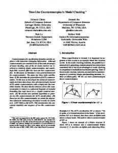
PJ6 PJ17 PJ18 heap 4

time (s)

10

3

10

2

10

1

4

8

16

32

64

processes

Fig. 5.

Time for multiple processes

within 1800 seconds; but BDD-based model checking requires at most a few seconds for each [9]. C. Results Table I reports results for executing one process on one processor of a 4×1.8GHz computer with 8GB of available memory. The analysis ran 16 times on each benchmark: Table I reports the number of variables in the cone of influence and the mean and standard deviation (in format mean (std. dev.)) for the number of discovered clauses, the number of SAT queries made, the required time, and the peak memory usage. Results are reported only for the nontrivial benchmarks: properties of benchmarks 0, 1, 4, 11, 12, and 14 of the PicoJava II set and benchmarks 3, 4, 7, 8, and 9 of the VIS PPC60x 2 set are inductive. The PicoJava II benchmarks are labeled PJx ; the others are VIS benchmarks. All 20 of the PicoJava II benchmarks were solved; three required more than one hour.

Figure 5 reports results as a log-log plot for analyzing PicoJava II benchmarks 6, 17, and 18 and VIS benchmark HEAP with multiple processes on a cluster of computers with 4×1.8GHz processors and 8GB of memory. Results for one processor are the means from Table I. Times for 32 processes are as follows: PJ6 , 8m; PJ17 , 70m; PJ18 , 9m; and HEAP, 6m. PJ17 completed in 50m with 60 processes. All benchmarks completed within one hour with some number of processes. The plot suggests that time decreases roughly linearly with more processes, but only HEAP trades processes for time almost perfectly, possibly because it requires the most clauses. Suboptimal scaling results from generating redundant clauses. VI. R ELATED W ORK A. Qualitative Comparisons We compare the characteristics of several safety analyses: bounded model checking (BMC) [15], interpolation-based model checking (IMC) [12], [13], k-induction (kI) [7]–[9], [16], [17], predicate abstraction with refinement (CEGAR) [18], [19], and our analysis (FSIS). These analyses are fundamentally based on computing an inductive set that excludes all error states; they consider the property to prove during the computation; and they use a SAT solver as the main computational resource. We now consider their differences. 1) Abstraction: IMC and CEGAR compute successively finer approximations to the transition relation. Each approximation causes a certain set of states to be deemed reachable. When this set includes an error state, IMC increments the k associated with its postcondition operator, solving larger BMC problems, while CEGAR learns a separating predicate. In contrast, BMC, kI, and FSIS operate on the full transition relation. kI strengthens by requiring counterexamples to induction to be ever longer paths. FSIS generalizes from CTIs to inductive clauses to exclude portions of the state space. 2) Use of SAT Solver: BMC, IMC, and kI pose relatively few but difficult SAT problems in which the transition relation is unrolled many times. CEGAR and FSIS pose many simple SAT problems in which the transition relation is not unrolled. 3) Intermediate Results: Each major iteration of IMC and CEGAR produces an inductive set that is informative even when it is not strong enough to prove the property. Each successive iteration of FSIS produces a stronger formula that excludes states that cannot be reached without previously violating the property. Intermediate iterations of BMC and kI are not useful, although exceptions include forms of strengthening, which we discuss in greater depth below [7]–[9], [17]. 4) Parallelizable: Only FSIS is natural to make parallel. The difficulty of subproblems grows with successive iterations in BMC, IMC, and kI so that parallelizing across iterations is not useful. Each iteration of CEGAR depends on previously learned predicates. For these analyses, parallelization must be implemented at a lower level, perhaps in the SAT solver. Differences suggest ways to combine techniques. For example, the key methods of FSIS and kI can be combined, and FSIS can serve as the model checker for CEGAR.

B. Other Related Work Blocking clauses are used in SAT-based unbounded model checking [5]. Their discovery is refined to produce prime blocking clauses, requiring at worst as many SAT calls as literals [6]. Our minimal algorithm requires asymptotically fewer SAT calls. A similar algorithm has been proposed in a different context [20], but it handles only sets containing precisely one minimal satisfying subset. Strengthening based on under-approximating the states that can reach a violating state s is applied in the context of k-induction [7]–[9], [17]. Quantifier-elimination [7], ATPGbased computation of the n-level preimage of s [8], and SAT-based preimage computation [9] are used to perform the strengthening. Inductive generalization can eliminate exponentially more states than preimage-based approaches. VII. D ISCUSSION Let us consider the methods of this paper more generally. The fundamental idea is to generalize from counterexamples to induction (CTIs) to simple inductive invariants. Together, the set of simple inductive invariants strengthens the specification to be inductive. Limiting the form of invariants controls computational costs, while using CTIs focuses the analysis on the safety specification. The structure of the analysis allows a parallel implementation. Two questions are immediate. What are the CTIs? What is the abstract domain for invariant generation? When the invariant generation is based on propagation, as in this paper, these questions are linked: the abstract domain should be conjunctive with respect to the CTI so that the best overapproximation to the CTI in the domain is sufficiently precise. For example, in FSIS, the CTIs are (partial) states that can lead to violations of the given property; and the domain consists of clauses of system variables. Clauses are conjunctive with respect to states like CTIs that ought to be unreachable. We thus start with Π and conjoin invariant clauses to exclude error states until CTIs no longer exist. As another example, consider the dual analysis in which the set of reachable states is grown until it is inductive without including any ¬Π-states. Now, the CTIs are (partial) states that are reachable in one step from the currently reachable set; and the abstract domain is cubes, which are conjunctions of literals. Hence, the invariant cubes are combined through disjunction to grow the reachable set. Each round of invariant generation discovers a minimal inductive subcube of the cube defined by the CTI that includes only Π-states. In another application, we explored inductive generalization from CTIs to affine inequalities [21]. In the domain of the analysis, invariant generation is not based on propagation. Once the form of the CTI and the abstract domain are fixed, one desires to find a greatest inductive generalization to each CTI. Standard techniques suggest how to perform one direction of propagation in the abstract domain [2]. However, the other direction must suffer from the nondeterminism inherent in over- (under-) approximating in a disjunctive (conjunctive) domain, so that a greatest inductive generalization

to the CTI need not be unique. For example, implicate is nondeterministic; and in the dual analysis, computing a best implicant is nondeterministic. The function minimal of Section IV-B is a general operator for performing forward (backward) propagation in disjunctive (conjunctive) domains. This general perspective on the ideas of this paper suggests further work in the form of exploring other domains. Additionally, we intend to combine the method with k-induction. Finally, our analysis is motivated by a classically deductive approach to verification [1]. We are exploring analyses for other classes of temporal properties that are also motivated by classically deductive techniques. ACKNOWLEDGMENTS The authors wish to thank Prof. A. Aiken, A. M. Bradley, Prof. E. Clarke, Prof. D. Dill, Dr. A. Gupta, Dr. H. Sipma, Prof. F. Somenzi, and the anonymous reviewers for their comments; and Prof. A. Aiken for the use of his computer cluster. R EFERENCES [1] Z. Manna and A. Pnueli, Temporal Verification of Reactive Systems: Safety. New York: Springer-Verlag, 1995. [2] P. Cousot and R. Cousot, “Abstract interpretation: a unified lattice model for static analysis of programs by construction or approximation of fixpoints,” in POPL. ACM Press, 1977, pp. 238–252. [3] B. Knaster, “Un theoreme sur les fonctions d’ensembles,” Ann. Soc. ¯ 133–134, 1928. Polon. Math., vol. 6,¯ pp. [4] A. Tarski, “A lattice-theoretical fixpoint theorem and its applications,” Pacific Journal of Mathematics, vol. 5, no. 2, pp. 285–309, 1955. [5] K. L. McMillan, “Applying SAT methods in unbounded symbolic model checking.” in CAV, ser. LNCS, vol. 2404. Springer, 2002, pp. 250–264. [6] H. Jin and F. Somenzi, “Prime clauses for fast enumeration of satisfying assignments to boolean circuits,” in DAC. ACM Press, 2005. [7] L. de Moura, H. Ruess, and M. Sorea, “Bounded model checking and induction: From refutation to verification,” in CAV, ser. LNCS. Springer, 2003. [8] V. C. Vimjam and M. S. Hsiao, “Fast illegal state identification for improving SAT-based induction,” in DAC. ACM Press, 2006. [9] M. Awedh and F. Somenzi, “Automatic invariant strengthening to prove properties in bounded model checking,” in DAC. ACM Press, 2006. [10] M. W. Moskewicz, C. F. Madigan, Y. Zhao, L. Zhang, and S. Malik, “Chaff: Engineering an Efficient SAT Solver,” in DAC, 2001. [11] K. L. McMillan and N. Amla, “Automatic abstraction without counterexamples.” in TACAS, ser. LNCS, vol. 2619. Springer, 2003, pp. 2–17. [12] K. L. McMillan, “Interpolation and SAT-based model checking,” in CAV, ser. LNCS, vol. 2725. Springer, 2003, pp. 1–13. [13] ——, “Applications of Craig interpolants in model checking.” in TACAS, ser. LNCS, vol. 3440. Springer, 2005, pp. 1–12. [14] VIS. [Online]. Available: http://visi.colorado.edu/∼ vis [15] A. Biere, A. Cimatti, E. M. Clarke, and Y. Zhu, “Symbolic model checking without BDDs,” in TACAS. Springer, 1999, pp. 193–207. [16] M. Sheeran, S. Singh, and G. Stalmarck, “Checking safety properties using induction and a SAT-solver,” in FMCAD, ser. LNCS, vol. 1954. Springer, 2000. [17] R. Armoni, L. Fix, R. Fraer, S. Huddleston, N. Piterman, and M. Vardi, “SAT-based induction for temporal safety properties,” in BMC, 2004. [18] E. Clarke, O. Grumberg, S. Jha, Y. Lu, and H. Veith, “Counterexampleguided abstraction refinement for symbolic model checking,” J. ACM, vol. 50, no. 5, pp. 752–794, 2003. [19] H. Jain, D. Kroening, N. Sharygina, and E. M. Clarke, “Word level predicate abstraction and refinement for verifying RTL verilog.” in DAC, 2005. [20] A. Zeller, “Yesterday, my program worked. Today, it does not. Why?” in ESEC / SIGSOFT FSE, 1999, pp. 253–267. [21] A. R. Bradley and Z. Manna, “Verification constraint problems with strengthening,” in ICTAC, ser. LNCS, vol. 3722. Springer, 2006.