Checking Semantical Consistency based on Observational Simulations Vlad Rusu* — Dorel Lucanu** * Inria Rennes Bretagne Atlantique Campus de Beaulieu 35042 Rennes Cedex, France
[email protected] ** Department of Computer Science
Alexandru Ioan Cuza University Iasi, Romania
[email protected]@ro We study the semantical consistency between two operational specifications of systems at two different levels of abstraction. We propose the notion of observational simulations to compare systems specified in terms of observational transition systems. We give a procedure for automatically detecting the absence of observational simulations between two observational transition systems (hence, their semantical inconsistency). The procedure also automatically finds executions of one specification that simulate a given execution of the other specification. ABSTRACT.
RÉSUMÉ. Nous nous intéressons ici à la cohérence sémantique entre deux spécifications opérationnelles d’un même système, situées à deux niveaux d’abstraction différents. Nous proposons la notion de simulations observationnelles pour comparer les systèmes spécifiés en terme de systèmes de transitions observationnels. Nous donnons une procédure qui permet de détecter l’inexistence d’une simulation observationnelle entre deux systèmes de transitions observationnels donnés (et donc, leur incohérence sémantique). Notre procédure détecte également des exécutions d’une des spécifications qui simulent une exécution donnée de l’autre spécification. KEYWORDS:
semantical consistency, observational simulations
MOTS-CLÉS :
cohérence sémantique, simulations observationnelles
1. Introduction and Motivation Assume that one wants to build a complex and critical embedded system. A reasonable approach is to first give a high-level description, expressed in a dedicated language such as, e.g., MARTE. From this high-level description, a lower -level de-
2
SafeModel track of IDM 2010.
High Level (e.g., MARTE) Consistency?
Low Level (e.g., SYSTEM C)
Figure 1. Semantical consistency. scription of the system can be generated, e.g., using model transformations - for example, the lower-level description of the system could written in SYSTEM C. (We mention embedded systems, the MARTE and SYSTEM C languages, and model transformations, to motivate our approach - the approach is not limited only to these technologies.) A natural question that arises is whether the two representations of the system are semantically consistent: do the executions of one level "match" with the executions of the other one? And if this is the case, with which ones? Also, higher-level and lower-level executions may have different "granularities" - one step at one level may correspond to several steps at the other level. Then, what does "matching" of executions mean? This paper proposes a tentative formal framework and solutions for these problems. The paper is organised as follows. In Section 2 we define observational transition systems and observational simulations as general, abstract models for, respectively, the executions of systems, and the "matching" between those executions. Then, semantical consistency amounts to checking whether an observational simulation between two given observational transition systems exists; and, if this is the case, to compute one. To solve these problems, we propose a construction called a simulation tree over two observational transition systems. We show that a certain condition on the simulation tree is equivalent to the existence of an observational simulation between the two observational transition systems (from which the simulation tree was constructed). This provides us with a procedure for automatically detecting the inexistence of an observable simulation, by exploring the simulation tree up to a finite depth. The procedure can also be used to find executions of one system that simulate a given, finite execution of the other one. In our hypothetical embedded-system design, executions obtained by emulating a SYSTEM C description of an embedded system could be "traced back" to the higher-level MARTE description; hence, if the emulation revealed an error, our procedure traces the error back to the high-level description, enabling users to fix it. In Section 3 we present related and future work and conclude.
2. Observational Transition Systems and their Observational Simulations Definition 1 (Observational Transition System (OTS) [OGA 08]) An OTS is a tuple hA, a0 , →, O, ωi where A is a nonempty, possibly infinite set of states; a0 ∈ A is the initial state; → ⊆ A×A is the (total) transition relation; O is a nonempty, possibly infinite set of observations; and ω : A → O is the observation function.
3
A:
a0
a1
B:
b0
b00
b1
b01
Figure 2. Two observational transition systems A, B with observation set {0, 1} and observation functions defined by ωA (ai ) = ωB (bi ) = ωB (b0i ) = i, for i = 0, 1. That is, observational transition systems are just transition systems, together with an observation domain and an observation function mapping states to observations. The following notions are rather standard for transition systems: an execution is a possibly infinite sequence of states π = a0 , ...an , ... such that for ai → ai+1 for i = 0, 1, ..., For technical reasons we also consider executions that start in states different from the initial state. For a finite execution π, we denote its length by len(π). Also, for a state a, we denote by exec(a) the set of executions π such that π(0) = a. Definition 2 (Matching, inspired from [MAR 08]) For two observational transition systems A = (A, a0 ,→A ,O,ωA ) and B = (B, b0 , →B , O, ω B ) having the same observation set O, and for two executions π of A and ρ of B, we say that π is Omatched by ρ if there exist two strictly increasing functions α, β : N → N such that α(0) = β(0) = 0, and such that for all i, j, k ∈ N, α(i) ≤ j < α(i + 1) and β(i) ≤ k < β(i + 1) imply ω B (ρ(j)) = ω A (π(k)). Example 1 Consider in Fig. 2 and the (unique) infinite executions π ∈ exec(a0 ) and ρ ∈ exec(b0 ). Then, each of these executions is {0, 1}-matched by the other one. Definition 3 (Observational Simulation) For observational transition systems A = (A, a0 , →A , O, ω A ) and B = (B, b0 , →B , O, ω B ) and states a ∈ A, b ∈ B, we say that a is observationally simulated by b, denoted by a -O b, if for all π ∈ exec(a), there exists ρ ∈ exec(b) such that ρ O-matches π. We say that A is observationally simulated by B, denoted by A -O B, if their initial states a0 , b0 satisfy a0 -O b0 . Example 2 Each of the observational transition systems A, B in Figure 2 is observationally simulated by the other one - based on the matching executions in Example 1. Next, we propose a contruction called a simulation tree and study its properties. Definition 4 (Simulation Tree) Given two observational transition systems A = (A, a0 , →A , O, ω A ) and B = (B, b0 , →B , O, ω B ), the simulation tree of A by B is the tree TA,B whose root r, set of nodes N , and set of edges E, are defined as follows: – r = ha0 , {b0 }i if ω A (a0 ) = ω B (b0 ), r = ha0 , ∅i otherwise – N ⊆ {ha, S}i ∈ A × P(B) | ∀b ∈ S.ω B (b) = ω A (a)}; – E and N are the smallest sets satisfying the following conditions:
4
SafeModel track of IDM 2010.
- if ha, Si ∈ N , a →A a ˆ, and ω A (ˆ a) = ω A (a), then hˆ a, Si ∈ N and (ha, Si, hˆ a, Si) ∈ E; - if ha, Si ∈ N , a →A a ˆ, and ω A (ˆ a) 6= ω A (a): let Sˆ = {ˆb ∈ B|∃b ∈ S.∃ρ ∈ exec(b).ρ(len(ρ)) = ˆb ∧ ω A (ˆ a) = ω B (ˆb) ∧ ∀k ∈ {0..len(ρ)−1}.ω B (ρ(k)) = ω B (b)}. ˆ ∈ N and (ha, Si, hˆ ˆ ∈ E. Then, hˆ a, Si a, Si) For example, in Figure 2 the simulation tree of A by B starting at (a0 , b0 ) is a linear sequence infinitely repeating the pattern ha0 , {b0 }i − ha1 , {b1 }i. In general, the nodes of a simulation tree TA,B have the form ha, Si, satisfying the invariant that all the states in their second component : b ∈ S, have the same observations as the state in their first component a. As usual in trees, the are edges from each node to its children; the children of a node "say" what the automaton B "does" when the automaton A "makes" a step, depending on whether the destination of the step has the same observation as its origin, or not. Accordingly, the set of children of a node ha, Si is the union of: – the set of nodes hˆ a, Si such that a →A a ˆ and ω A (ˆ a) = ω A (a); here, the first component a ˆ is obtained by taking one execution step from a, and it has the same observation as a; then, the second component S remains unchanged. Note that this is enough to preserves the above-mentioned tree invariant regarding observations. ˆ such that a →A a – the set of nodes hˆ a, Si ˆ and ω A (ˆ a) 6= ω A (a): now, a ˆ is obtained by one execution step from a, but its observation is different from that of a. Then, the transition system B "builds" the set Sˆ by taking executions ρ from states ˆ such that (i) the observation of ˆb equals the "new" b ∈ S to states ˆb = ρ(len(ρ)) ∈ S, observation ω A (ˆ a), and (ii) ρ does not have a proper subsequence with that property. Note that this also preserves the tree invariant on nodes regarding observations. Note also that such states ˆb may not exist, in which case the resulting node is hˆ a, ∅i. These observations are formalised in the following theorem - the paper’s main result. Theorem 1 For observational transition systems A, B, A -O B iff for all nodes ha, Si of TA,B , S 6= ∅. Moreover, for any execution π of A, consider the path of the form (hπ(i), Si i)i≥0 in TA,B , whose projection on its first component is π. Then, all executions ρ of B satisfying the condition ρ(i) ∈ Si for all i ≥ 0 are O-matches for π. The theorem contains two statements. The first one naturally suggests a procedure for detecting the absence of an observational simulation: explore a finite prefix of TA,B - since TA,B is infinite, in general - and stop if node of the form ha, ∅i is found; we say the simulation tree found a counterexample. An equivalent, optimised procedure consists in stopping the exploration when a node of the form ha0 , S 0 i is encountered during the exploration, and there already is a node ha0 , Si with S ⊆ S 0 in the tree, and a path from ha0 , Si to ha0 , S 0 i. This is because the set S of states of B possibly simulating a0 can only grow, and S is already nonempty - otherwise the exploration would have already stopped at ha0 , Si. We say the simulation tree found a circularity. (Such counterexamples and circularities are illustrated on a simple example below.)
5
Probably the most useful practical application of this work is finding executions of B that match a given finite execution of A, as discussed at the end of Section 1. The second statement in Theorem 1 says that the simulation tree can be used exactly for that purpose (actually, one only needs to build the finite, linear path (hπ(i), Si i)0≤i≤len(π) in the tree, which saves us an exponential blowup, making the procedure manageable). Note the if implication and the absence of the only if. The reason is that our simulation tree does not contain all sequences ρ of B matching a given sequence π of A (but if there is a matching sequence, at least one will be represented in the simulation tree). To further illustrate simulation trees we represent in Fig. 3 a simple program, together with three observational transition systems generated from it. Their observation functions, are, from left to right: the set of program counter values in which the program may be at a given time; the (single) program counter value in which the program may be; and the program counter value, together with the positiveness/negativeness of x. // x > 0 if (1) x > 5 → x := x + 5; (2) x < 10 → x := x + 10; fi do (3) odd(x) → x := −3 ∗ x; (4) even(x) → x := x/2; (5) x ≤ 0 → x := −x + 3; od
Figure 3. A nondeterministic program, and three observational transition systems. We denote the three observational transitional system by A, B, C from left to right. Figure 4 depicts the simulation trees TA,C and TB,C . The former detects a circularity, and illustrates the fact that C observationally simulates A. The latter detects a counterexample, and illustrates the fact that C does not observationally simulate B.
3. Conclusion, Related work, and Future Work We present a formal framework and some initial solutions to the problem of checking semantical consistency between two operational specifications of a system at two different levels of abstraction. The framework involves a notion of observational simu-
6
SafeModel track of IDM 2010.
Figure 4. Simulation trees: (left) C simulates A
(right) C does not simulate B.
lations between observational transition systems, and the definition of simulation trees that encode observational simulations between observational transition systems. Due to space limitations we only cite here a few related works. Simulations in general are well-known in the area of formal verification; various forms of simulations are discussed in the book [CLA 99]. A general form of simulations, called stuttering simulations, is studied in an algebraic setting in [MAR 08]. Our observational simulations are a particular case of stuttering simulations, tailored to the model of observational transition systems. A richer model of observational transition systems (over an algebraic signature) is employed in [OGA 08], and inductive theorem proving is used to check whether a given relation between states of such systems is a simulation. Our approach is different: we automatically compute (currently, only up to a bounded number of steps) the simulations between two observational transition systems; this allows us to effectively find matching executions between two specifications. In future work we shall use the circular coinduction proof technique implemented in the CIRC theorem prover [LUC 09] to compute observational simulations.
4. References [CLA 99] C LARKE E. ., G RUMBERG O., P ELED D., Model Checking, MIT Press, 1999. [LUC 09] L UCANU D., G ORIAC E.-I., C ALTAIS G., ROSU G., “CIRC: A Behavioral Verification Tool Based on Circular Coinduction”, K URZ A., L ENISA M., TARLECKI A., Eds., CALCO, vol. 5728 of Lecture Notes in Computer Science, Springer, 2009, p. 433-442. [MAR 08] M ARTÍ -O LIET N., M ESEGUER J., PALOMINO M., “Algebraic Stuttering Simulations”, Electr. Notes Theor. Comput. Sci., vol. 206, 2008, p. 91-110. [OGA 08] O GATA K., F UTATSUGI K., “Simulation-based Verification for Invariant Properties in the OTS/CafeOBJ Method”, Electr. Notes Theor. Comput. Sci., vol. 201, 2008, p. 127-154.