Checking Untimed and Timed Linear Properties of the Interval Timed Colored Petri Net Model Verificación de las propiedades lineales síncronas y asíncronas del Modelo de la Red de Petri Coloreado Intervalo Tiempo Hanifa Boucheneb Department of Computer Engineering, École Polytechnique de Montréal, P.O. Box 6079, Station Centre-ville, Montréal, Québec
[email protected]
Article received on July 30, 2004; accepted on December 11, 2006 Abstract This paper deals with verification of timed and untimed linear properties of the Interval Timed Colored Petri Net model. This model can simulate other timed colored Petri nets and allows describing large and complex real-time systems. We propose here to contract its generally infinite state space into a graph that captures all linear properties of the model. The resulting graph is finite iff, the model is bounded (the set of its reachable markings is finite). In this case, linear properties of the model can be verified on the graph using, for example, the classical linear model checking techniques. Keywords: Formal methods, model checking, timed models, timed colored Petri net, state space contraction, linear properties. Resumen Este artículo se ocupa de la verificación de las propiedades lineales temporizadas y no temporizadas del modelo de redes de Petri coloreadas con intervalos temporizados. Este modelo puede simular otras redes de Petri coloreadas temporizadas y permite describir grandes y complejos sistemas en tiempo real. Nosotros proponemos contraer el espacio generalmente infinito, en un grafo que capture todas las propiedades lineales del modelo. El grafo resultante es finito, si y solamenti si, el modelo tiene límites (el conjunto de sus marcas accesibles es finito). En este caso, las propiedades lineales del modelo se pueden verificar en el grafo resultante, utilizando, por ejemplo, técnicas de comprobación del modelo lineal clásico. Palabras clave: Métodos formales, comprobación modelo, modelos temporizados, red de Petri coloreada con intervalos temporizados, contracción del espacio del estado, propiedades lineares.
1 Introduction Verification of concurrent systems is a complex task that requires powerful models and efficient analysis techniques. Model checking is one of the most popular verification techniques of concurrent systems [1, 2, 3, 11, 12, 15]. In this technique, the behavior of a system is represented by a finite transition system (state graph or state space), and the properties to be verified are expressed in either a standard temporal logic (LTL, CTL, CTL*) [1, 2, 12, 21], or in its time extension (MITL, TCTL) [1, 2, 18]. Properties are checked by exploring the state graph (an enumerative method). In theory, the applicability of this method is restricted to finite graphs, but in practice, it also runs up against the state explosion problem. To overcome these limitations, one solution consists in contracting the state graph into a finite and compact structure allowing to verify properties of interest [3, 4, 5, 6, 7, 8, 9, 10, 11, 13, 14, 16, 18, 19, 20, 21]. This paper aims to apply the linear model checking techniques for timed colored Petri nets. Colored Petri nets (CPNs) are successfully used to specify and analyze complex systems. In this model, a color (a value) is associated with each token allowing to make much compact and manageable descriptions. To be able to analyze systems whose behaviors are time dependant, several extensions to time parameter have been proposed for the CPN model (Van der Aalst in [19], Christensen in [10], Pao-Ann Hsiung [16]). In Pao-Ann Hsiung's model, a time interval is associated with each transition specifying its minimal and maximal firing delays. Time intervals of this model have the same semantics
Computación y Sistemas Vol. 10 No. 2, 2006, pp 107-134 ISSN 1405-5546
108
Hanifa Boucheneb
as those of Merlin's model (Time Petri Nets) [5]. In Christensen's model, a date is associated with each created token, which indicates when the token will become available. An enabled transition will occur as soon as possible (when all its required tokens become available). The Van der Aalst's model called Interval timed Colored Petri Net (ITCPN) associates with each created token a time interval specifying when the token will become available (the earliest and latest times). As in Christensen's model, an enabled transition will occur as soon as possible. Among these extensions, the model proposed by Van der Aalst seems to be more appropriate since time intervals are associated with tokens instead of transitions or places. But, unlike Pao-Ann Hsiung's model, the Van der Aalst's model does not allow unbounded intervals and then expressing that a created token could be never available (be lost) is not possible. To overcome this limitation, we extend this model by allowing unbounded intervals. With this extension, the model can simulate other timed colored Petri nets and allows describing, in a concise way, large and complex real-time systems. However, because of time density, the ITCPN state space is generally infinite. Therefore, its analysis by enumeration needs an extra step to contract its state space into a finite graph preserving properties of interest (linear properties: LTL, MITL). We say that a graph preserves linear properties of some model, if we can determine from it all evolutions of the model. Van der Aalst proposed in [19], a contraction method for the ITCPN model which is "sound" (i.e.: any occurrence sequence in the state space of the model is also possible in the contracted state space) but not "complete" (i.e.: some firing sequence in the contracted state space does not reflect any firing sequence in the model state space). Therefore, the contracted space has not necessarily the same linear properties as the model. Moreover, for models allowing infinite firing sequences, theVan der Aalst's method produces infinite graphs. We propose here another contraction approach that generates finite graphs for all bounded ITCPNs. Our approach is both "sound" and "complete" and the resulting graph preserves all linear properties of the model. It can be used to verify linear properties of the model. Untimed linear properties can be verified using the standard linear model checking techniques. To verify timed linear properties, we generally need to compute the minimal and maximal executing times of some firing sequences (paths of the graph). We develop here an algorithm that computes for a given path of the graph, its minimal and maximal path times. Firstly, we give, in section 2, some definitions related to the ITCPN model and its behavior. We show afterwards, in sections 3, 4 and 5, how to contract the ITCPN state space into a graph preserving linear properties of the model. We distinguish two levels of contraction. In the first level (section 3), we agglomerate into one state class, all states reachable by firing the same sequence independently of their firing dates. Section 4 is devoted to the simplification of the firing rule given in section 3. We establish here an attractive characterization of state classes that simplify considerably their computation and their comparison. Afterwards, we show by means of an example that this contraction can produce infinite graphs for some bounded ITCPNs. For further contractions, we propose, in section 5, to relax state classes. In section 6, we show that with this relaxation, we obtain finite graphs for all bounded ITCPNs. Section 7 shows how to compute path times. Section 8 is devoted to an application example.
2 The Interval Timed Colored Petri Net model The ITCPN model is a colored Petri net (CPN) augmented with time intervals associated with tokens. From the semantic point of view, each created token has a time stamp which can be any value inside its associated interval. The time stamp of a token indicates the delay required for the token to become available. 2.1 Formal definition of the ITCPN model We introduce here only necessary definitions and notations. For further details, we refer to [17] for CPNs and to [19] for ITCPNs. Definition 1: (Time domain, multisets)
Computación y Sistemas Vol. 10 No. 2, 2006, pp 107-134 ISSN 1405-5546
Checking Untimed and Timed Linear Properties of the Interval Timed Colored Petri Net Model
-
109
The time domain is the set of all non-negative real numbers plus ∞ , i.e.: R+ ∪ {∞}. Note that ∞ is considered here as a particular value which satisfies the following relations: r+∞ = ∞+r=∞, r ≤ ∞, for each r ∈ (R+ ∪ {∞}), and ∞∞ = ∞. Let X be a set. A multiset over X is a function N which associates with each element of X, an integer number. It is represented by the formal sum: ∑x∈ X N(x)•x, where N(x) is the occurrence number of x in N. Let X be a set, N1 and N2 two multi-sets over X. Operators +, - , ≤, = on multi-sets are defined as usual: o N1 + N2 = ∑ x∈ X (N1(x)+N2(x))•x. o N1 ≤ N2 iff, ∀x∈ X, N1(x) ≤ N2(x). o N1 = N2 iff, ∀x∈ X, N1(x) = N2(x). o if N1 ≤ N2 then N1 - N2 = ∑x∈X (N1(x)-N2(x))•x. o The size of N1 denoted by |N1| is: ∑x∈X N(x). We denote by XMS the set of all multisets over X, and by 0 or ∅ the empty multiset.
-
Definition 2: (ITCPN model) An ITCPN is a tuple ( ∆, P, T, C, F, TM0 ) where: ∆ is a finite set of color sets. Each color set is finite. P is a finite and non empty set of places. T is a finite set of transitions such that: (P∩ T = ∅). Cd: P → Powerset(∆)1. Cd(p) ∈ Powerset(∆), is a finite set of all allowed colors in place p. Let CT be the set of all possible colored tokens, i.e.: CT = {(p, c) | p ∈ P ∧ c ∈ Cd(p)} and INT the set of all intervals defined by: {[y,z] ∈ Q+ × (Q+ ∪ ∞) | y ≤ z}. Note that unlike Van der Aalst's model, we allow here unbounded intervals. F is the transition function over T. F(t): Dom(F(t)) → (CT × INT)MS, where Dom(F(t)) ⊆ CTMS. F(t) specifies which tokens are consumed and produced by firing transition t. It also specifies the time stamp intervals of the created tokens. Each transition is supposed to produce a finite set of tokens. TM0 is the initial marking indicating which tokens are present initially, their colors and their time stamps, i.e.: TM0 ∈ (CT × (Q+∪ {∞})MS.
-
-
2.2 ITCPN behavior We first explain the behavior of the model, using an example given in [19] and reported here in Figure 1.
Fig. 1. An ITCPN model of a Jobshop 1
Powerset(∆) is a set such that ∆⊆ Powerset(∆) and ∀ A,B∈ Powerset(∆), A×B∈ Powerset(∆).
Computación y Sistemas Vol. 10 No. 2, 2006, pp 107-134 ISSN 1405-5546
110
Hanifa Boucheneb
Figure 1 is the graphic representation of an ITCPN composed of three places {pin, pbusy, pfree}, two transitions t1, t2 and three color sets: - M = {M1, M2,..., Ms} associated with place pfree, - J = {J1, J2,.., Jr} associated with place pin, and - M × J associated with place pbusy. It represents a jobshop, where jobs of place pin are executed repeatedly. The jobshop is composed of one or several machines. Each machine is represented by a token, which is either in place pfree or in place pbusy. Tokens consumed and produced by firing transitions t1 and t2 are specified by functions F(t1) and F(t2) defined by: - ∀ j ∈ J, ∀ m ∈ M, F(t1)((pin, j) + (pfree, m)) = (pbusy, (m, j), [1,3]). F(t1) means that transition t1 consumes one token from each place pin and pfree , and produces one token in place pbusy. When transition t1 occurs, the time stamp of the created token can be any value inside interval [1,3]. ∀j ∈ J, ∀m ∈ M , F(t2)((pbusy, (m, j))) = (pfree,m, [2,2]) + (pin, j, [1,1]). F(t2) means that transition t2 consumes one token from pbusy and produces two tokens one in each place pin and pfree. When transition t2 occurs, the time stamps of the tokens created in places pfree and pin are respectively 2 and 1. Initially, there are three tokens: TM0=(pfree, M1,2)+(pin,J1,1)+(pin,J2,2). 2.2.1 States of an ITCPN To characterize the model state, we associate with each token a variable, called clock, which measures the time elapsed since the creation of the token. The clock is initialized to 0, when the token is created. Afterwards, its value increases synchronously with time until its associated token is consumed. -
Definition 3: (Timed tokens, states) A timed token is a tuple (p,c,v,[a,b]) where p is its place, c is its color, v is its clock value (or its clock name) and [a,b] is its time stamp interval. A state σ of an ITCPN is a multi-set of timed tokens, i.e.: σ ∈ (CT × R+ × INT)MS. The initial state of an ITCPN is obtained from its initial timed marking TM0 by completing appropriately each token.
Note that there are other state definitions used in [6, 7, 19]. In [6, 7], a variable, called delay, is associated with each token indicating the time to wait before the token becomes available. When a token is created, its delay is initialized to any value inside its time stamp interval. Afterwards, its value decreases with time until its associated token disappears. Delays are less appropriate than clocks to verify timed properties. The verification of these properties generally needs to compute some path times. The computation of path times is simpler using clocks, as they measure the time elapsed since they are initialized to zero. In [19], each token is completed with a date interval indicating the minimal and maximal dates at which the token will become available. If a token is created at date τ, its date interval is [a+τ, b+τ], where [a,b] is its time stamp interval. This state definition is not appropriate for enumerative methods, since for models allowing infinite firing sequences, the date will grow infinitely leading to infinite graphs. 2.2.2 State evolution Initially, the model is in its initial state. Afterwards, its state evolves either by time progressions (clocks increase with time) or by firings. Definition 4: (State events) Computación y Sistemas Vol. 10 No. 2, 2006, pp 107-134 ISSN 1405-5546
Checking Untimed and Timed Linear Properties of the Interval Timed Colored Petri Net Model
111
Let σ be a state and M(σ) the marking obtained from σ by eliminating all time parameters (the underlying marking). - Let t be a transition of T. Transition t is enabled for σ iff all tokens required for its firing are present in σ , i.e.: ∃ m ∈ Dom(F(t)), m ≤ M(σ). - An event of σ is a pair (t,in) where t is an enabled transition for σ and in is all tokens participating in its enabling. - Let e be an event of σ. Jin(e) denotes the multi-set of timed tokens required for firing event e. We have: Jin(e) ≤ σ. - We denote E(σ) the set of all events of σ. - Two events e1 and e2 are conflicting for σ iff, Jin(e1) + Jin(e2) < σ. When an event is fired all event conflicting with it are disabled. In this model, an event shall occur as soon as possible (i.e.: when all required tokens become available). Its firing takes no time but leads to a new marking: consumed tokens disappear and possibly new tokens are created. Let σ be a reachable state of an ITCPN, ef=(tf,Jin(ef)) an event of σ and dv a non-negative real value. Definition 5: (Time progression) Let (p,c,v,[a,b]) be a token of σ. The delay interval of this token is the domain of the time required to become available, i.e.: [max(0,a-v),max(0,b-v)]. - Let e be an event of σ. The occurrence delay (i.e.: the firing delay) of e is the delay required for all tokens of Jin(e) to become available. The minimal and maximal firing delays of e denoted respectively by FDmin(e) and FDmax(e) are max(0, max(p,c,v,[a,b])∈Jin(e) (a - v)) and max(p,c,v,[a,b]) ∈ Jin(e) (b-v). From the semantic of the model (an event shall occur as soon as possible), there is at least one token (p,c,v,[a,b]) in Jin(e) such that v ≤ b holds. By convention, if Jin(e) is empty, FDmin(e) and FDmax(e) are equal to zero. - A time progression of dv units can occur from the state σ (without any firing) iff, dv is smaller or equal to the maximal firing delays of all events, i.e.: dv ≤ mine ∈ E(σ) FDmax(e). By convention, if E(σ) is empty, (mine∈E(σ)FDmax(e)) is equal to ∞. This condition of time progression is denoted σ→dv. - After this time progression, the clock of each token (p,c,v,[a,b]) of σ increases by dv time units. We denote (σ)+dv the reached state: ∑(p,c,v,[a,b])∈ σ σ(p,c,v,[a,b]) • (p,c,v+dv,[a,b]). We write σ→dv σ' iff the state σ' is reachable from σ by time progression of dv units. -
-
Definition 6: (Event firing) Event ef can occur immediately from σ (without any progression of time) iff, its minimal firing delay is equal to 0, i.e.: FDmin(ef) = 0. This immediate firing condition is denoted by σ→ef. If ef can occur immediately from σ, its occurrence is instantaneous and leads to the state σ' = σ - Jin(ef) + Jout(ef), where Jout(ef) is obtained from F(tf)(M(Jin(ef))) by completing each token with the initial value of its clock (i.e.: 0 ). Recall that F(tf) is the transition function of tf. This immediate firing is denoted by σ→ef σ'. Event ef can occur from σ after possibly some progression of time iff, its minimal firing delay is not greater than the maximal firing delays of all other events, i.e.: (FDmin(ef) ≤ mine∈E(σ) (FDmax(e))). If ef can occur from σ, it will occur after any delay dv inside interval [FDmin(ef), mine∈E(σ) FDmax(e)]. Its occurrence σ'= (σ - Jin(ef))+dv + Jout(ef). is instantaneous but leads to the state σ': An evolution of σ is a sequence of events and time progressions that can occur successively from σ. Evolutions of an ITCPN are those of its initial state.
Note that for the ITCPN model, the evolution of a state σ depends only on its underlying untimed tokens M(σ) and the delay intervals of its tokens. Example 1: (State evolution) Computación y Sistemas Vol. 10 No. 2, 2006, pp 107-134 ISSN 1405-5546
112
Hanifa Boucheneb
Consider the previous model (Figure 1). Its initial state σ0 consists of three tokens: (pfree,M1,0,[2,2])+(pin,J1,0,[1,1])+(pin,J2,0,[2,2]). The first and the third one will become available after two time units while the second one will become available after one time unit. State σ0 has two events: e1= (t1,(pfree, M1, 0, [2,2]) + (pin, J1, 0,[1,1])) and e2= (t1, (pfree, M1,0, [2,2]) + (pin, J2,0,[2,2])). Their minimal and maximal firing delays are: FDmin(e1)= FDmax(e1)= max(0,2-0,1-0) and FDmin(e2)= FDmax(e2)=max(0,2-0,2-0). Both events can occur from the initial state after 2 time units. After 2 time units, the model will reach the state: (pfree,M1,2,[2,2]) + (pin,J1,2,[1,1]) + (pin,J2,2,[2,2]). The occurrence of event e1 leads to the state σ1= (pin, J2,2,[2,2]) + (pbusy, (M1,J1),0,[1,3]). The occurrence of event e2 leads to the state σ2 = (pin, J1,2, [1,1]) + (pbusy, (M1,J2),0,[1,3]). Definition 7: (State space) The state space of an ITCPN is the graph of its evolutions. It is defined as a tuple (SS,→, σ0) where: - σ0 ∈ SS is the initial state; - → ⊆ (SS × (EE ∪ R+) × SS ) is the transition relation defined in Definitions 5 and 6, EE is the set of all events; - SS = { σ | σ0→∗ σ}, where →∗ is the reflexive and transitive closure of →. Because of time density, the state space of the ITCPN model is generally infinite and then not useful for enumerative analysis methods. Van der Aalst proposed in [19] a contraction method for the ITCPN state space which is "sound" but not "complete". This is due to the fact that this method “forgets” the occurrence time to memorize only intervals, i.e.: a state class (a set of states) is defined as a multiset of triplets of the form (place, color, interval). Consequently, for event producing several tokens, the dependencies (relations binding intervals) are lost and resulting classes may contain unreachable states (leading sometimes to unreachable markings). For instance, consider the model shown in Figure 2. We suppose that the color domain of each place is {e}, the initial state is (p0,e,0) and transition functions are defined as follows: F(t0 )((p0, e)) = ( p1, e,[0,2]). - F(t1)((p1, e)) = ( p2, e,[1,2]) + (p3,e, [1,3]). - F(t2)((p2, e)) = F(t3)((p3, e)) = 0. Using the Van der Aalst's method, the firing of transition t0 leads to the state class (p1,e,[0,2]). The firing of t1 from this class produces the class (p2,e,[1+0,2+2]) + (p3,e,[3+0,4+2]) where states (p2,e,1) +(p3,e,6) and (p2,e,4) +(p3,e,3) are represented but not reachable. From the former state, transition t2 is fired before t3 (1 < 6) while from the second, transition t3 is fired before t2.(3 < 4). Van der Aalst's method states that both markings (p2,e) and (p3,e) are reachable which is in fact wrong. The reason is that after firing transition t1, the created token (p2,e) becomes available before token (p3,e) ([1,2] F[0,4] (pbusy , (M1,J1)). This property means whenever the job J1 is waiting for execution, it must be in execution within 4 time units. To verify this property, we have to construct the synchronous product of the timed buchi automaton of the property and the state class graph shown in Figure 3. The part of the resulting graph, which exhibits that the synchronous poduct is not empty, is shown in Figure 6. The property is not satisfied since there exists a cycle which passes over the acceptation node (Err).
Fig. 6. A part of the synchronous product of the class graph and timed automaton shown resp. in Figures 3 and 5.
Computación y Sistemas Vol. 10 No. 2, 2006, pp 107-134 ISSN 1405-5546
Checking Untimed and Timed Linear Properties of the Interval Timed Colored Petri Net Model
129
Table 2 shows how to compute time bounds of the path (α0 init) e2 (α2 int) e4 (α24 int) which corresponds to the bounds of clock hp when the final node of the path is reached. Table2 Computing bounds of some path time
(α0 init)
H0(hp,o) = H0(hp,h1)= 0 H0(hp,h2)= H0(hp,h3) = 0 H0(o,hp)= H0(h1,hp) = 0 H0(h2,hp) = H0(h3,hp) = 0
(α2,int)
H2(hp,o) = H2(hp,h5)= 2; H2(hp,h2)= 0 ; H2(o,hp) = H2(h5,hp) =-2; H2(h2,hp)= ∞.
(α24 int)
H24(hp,o)= H24(hp,h1)= 5; H24(hp,h2)= 0; H24(hp,h3) = 5 ; H24(o,hp)= H24(h1,hp)= -3; H24(h3,hp)= -3; H24(h2,hp) = ∞
7 Application To illustrate our approach, we consider a more realistic example. In a hospital, each patient has a medical record composed of various informations (administrative, medical, surgical... etc). These informations can be stored within a single computer or distributed over a large number of interconnected systems. However, each user of the system should only access needed information for which he has the right clearance. For instance, a doctor needs to access information about his patient medical records. Whereas a secretary is only allowed to access administrative information such as the name, the age, costs of the treatments...etc. We then consider a decision-making system to decide whether or not a surgical operation is necessary according to patient state. Figure 7 shows the corresponding ITCPN model composed of seven places p1 , p2 , …, and p7, representing message channels and five transitions t1, t2, …, and t5 representing processes where:
-
p1 is a database containing all medical records of the hospital patients. These records should be accessed only by the director represented by t1. p2 is a database containing all the results of the analysis. The doctor which is represented by t3 is the only one who is authorized to have access to it. p3 is the administrative information channel of the secretary t2. p4 is the doctor's message channel. p5, p6 and p7 are the message channels of the surgeon t4 and t5.
Transitions are the active entities of the system. We associate with each transition t a function F(t) which describes the resources handled during its execution and those produced. In order to insure confidentiality and integrity of information within the system, we use the multilevel security model MLS proposed by Bell-LaPadula where security levels are assigned to the objects and subjects (users) of the system. Security requirement are characterized by two axioms: (a) No user may read information classified above his security level ("No read up"); Computación y Sistemas Vol. 10 No. 2, 2006, pp 107-134 ISSN 1405-5546
130
Hanifa Boucheneb
(b) No user may lower the classification of information ("No write down"). For our example, we consider the set of security classes SC={U (unclassified), C (confidential), S (secret)} with U ≤ C ≤ S. We link to each place the set of allowed security class in order to describe the clearance of the different subjects to various informations. This set is specified as its color domain. For this example, we suppose that: Cd(p1)= {U,C}, Cd(p2)= SC, Cd(p3)= {U}, Cd(p4)= {U,C}, Cd(p5)= {U}, Cd(p6)=SC, Cd(p7)= SC. So, the security classes {U, C} of p1 (director's channel) means that the director is authorized to handle only data of security classes C and U. For that, each information will have a security class which describes its confidentiality. We also need to define the information flow assertions through all transitions. For need to simplification, we assume the following security requirement such as information cannot be downgraded by a transition. This is to be applicable to all transitions except transition t5. Each transition will be linked by a function F defined by:
-
F(t1)((p1,E))= (p3, E, [1,2]) + (p4, E, [0,2]); F(t2)((p3,E))= (p6, E, [0,2]); F(t3)((p2, E) + (p4, E')) =(p5, max(E,E'), [1,3]); F(t4)((p5, E) + (p6, E')) =(p7, max(E,E'), [0,0]); F(t5)((p7, E)) = (p1, min(E,C), [0, ∞]) + (p2, E, [1,2]) where E, E' ∈ {U, C, S}. F(t1) means that when the director decides to treat a medical record of a patient with a security class E, he produces two data about this patient: - Administrative information that will be transferred to the secretary's channel. This information will have a time interval [1,2] and the security class of the consumed token. - Medical information intended for the doctor's channel. Time interval and security class of this information are respectively [0,2] and E. To simplify the explanation, we suppose that we have only one patient in each database (p1 and p2). The initial state class of the model is: α0 = (SM0, FT0), where: SM0 =(p1, C, h1, [0, ∞]) + (p2, S, h2, [0, ∞]) and FT0 = (h1 = 0 ∧ h2 =0).
Fig.7. Sample medical process
Computación y Sistemas Vol. 10 No. 2, 2006, pp 107-134 ISSN 1405-5546
Checking Untimed and Timed Linear Properties of the Interval Timed Colored Petri Net Model
131
Our interest is to verify some security properties such as integrity and confidentiality according to Bell-LaPadula's rules: "No Read up" and "No Write down". "No Read up" states that a low-level subject is not allowed to read highlevel objects while "No Write down" states that no user may lower the classification of information. Using LTL, these security requirements about states and flows can be expressed as follows: - Integrity: G (SecureState). This property means that all reachable states are secure. The proposition SecureState is evaluated to true for some state if and only if the security class of each token (p, c, h, [a,b]) of the state conforms with the security classes of its place (i.e. c ∈ Cd(p)). It is a general way to ensure integrity because it helps to verify that only authorized subjects are allowed to operate with the data in the system. - Confidentiality: G (SecureFlow). This property means that all flows are secure. The proposition SecureFlow is evaluated to true for some state if and only if the security class of each token conforms to the security classes of its place and is not smaller than the security classes of all tokens participating to its creation. In the state class graph, all states agglomerated within the same class share the same marking. Therefore, some state within a state class satisfies proposition SecureState iff, all states within the state class satisfy the proposition. By construction of the state class graph, if two state classes α and α’are connected by an arc then there is at least one state in α which leads by the arc to some state in α’. These two features of our state class graphs make them suitable to verify the security properties above. Hence the verification of these properties is performed on the state class graph by exploring its nodes and arcs and checking whether propositions SecureState and SecureFlow are satisfied not. As an example, consider the state class graph (Figure 8) of the model shown in Figure 7 and the state class α1=(SM1, FT1) reachable by firing event e1=(t1, (P1, C, h1, [0, ∞]) from the initial state: SM1= (p2, S, h2, [0,∞]) +(p3, C, h3, [1,2]) + (p4, C, h4, [1,2]), FT1 = (0 ≤ h2 ≤ ∞ ∧ h3 = 0 ∧ h4 = 0). States of this class are insecure because confidentiality and probably integrity of some information is compromised. Indeed, the security class of token deposited in the place p3 does not belong to the set of security classes admitted in this place, i.e.: C ∉ Cd(p3). This problem may result in a Read-up operation because the secretary may read information classified above her clearance level. Therefore, both properties G (SecureState) and G (SecureFlow) are not satisfied. Another problem concerns the arc (α5, t5, α0). This transition downgrades the security classes of information but is supposed to act as a filter process to remove parts of information that are not eligible to be received by a particular subject. It is defined in this way in order to prevent secret information to be handled by unauthorized subjects. Therefore, insecure information flows should occur only in the filter process of the system that is considered as a trusted component. Note that to verify both properties (and some others such as reachability and invariant), we can use an abstraction by inclusion to further attenuate the state explosion problem. When a state class is explored, there is no need to explore another state class which is included in it. During the construction process, classes are computed in the same way as in section IV, but when a new class is computed, we check for inclusion instead of equality. All classes such that one of them englobes the others are grouped together. In [9], authors have shown that abstraction by inclusion has a good impact on performances. Both computation times and graph sizes are reduced by a factor reaching hundred in certain cases. Another important feature of our state class representation is that it simplifies the test of inclusion. Indeed, a state class α =(SM,FT) is included in a state class α'=(SM',FT') iff, it is possible to rename clocks in (SM',FT') so as to obtain: SM = SM' and ∀(x,y) ∈ VSM2, H(x,y) ≤ H’(x,y). Table 3 compares graph sizes obtained with and without abstraction by inclusion for the model shown in Figure 7. We have considered different initial markings; parameter n is the number of patients in each database (i.e.: number of tokens initially in each place p1 and p2). Table 3 Using abstraction by inclusion
n
Using =
Using ⊆
Ratio Computación y Sistemas Vol. 10 No. 2, 2006, pp 107-134 ISSN 1405-5546
132
Hanifa Boucheneb
2 3 4 5
Nodes Arcs CPU(s) Nodes Arcs CPU(s) Nodes Arcs CPU(s) Nodes Arcs CPU(s)
193 430 0,01 7572 25956 0,97 358681 1681788 130,54 -
54 128 0 686 2466 0,10 11376 54949 3,7 232872 1414042 191,1
3,6 3,4 11 10,5 9,7 31,5 30,6 35,3
Fig. 8. The state class graph of the ITCPN of Figure 7
8 Conclusion This paper has considered the Interval Timed Colored Petri Nets (ITCPNs) proposed by Van der Aalst in [19]. This model allows to describe, in a concise way, large and complex systems, but due to time density, its state space is generally infinite and then not useful for model checking techniques. To apply the linear model checking techniques to this model, we have to contract its state space into a finite graph preserving linear properties of the model. In this way, linear properties of the model can be checked on the obtained graph using the classical linear model checking techniques. Van der Aalst proposed a contraction for the ITCPN state space which does not necessarily preserve the linear properties of the model. Moreover, this technique generates infinite graphs for models allowing infinite firing sequences. We developed here an efficient contraction which does not have these drawbacks. For bounded ITCPNs, our approach generates finite graphs which preserve linear properties. The resulting graphs are then useful to model check linear properties of the model. In addition, to deal with timed linear properties, we showed how to compute by exploring a path of the state class graph, the minimal and maximal times to execute the firing sequence of the path. Finally, we showed by means of an example how to verify using Büchi automata the timed linear properties. Note that we have considered here only equivalences based on clocks for further agglomerations, state class graphs can be more contracted with equivalences based on colors as shown in [6].
Computación y Sistemas Vol. 10 No. 2, 2006, pp 107-134 ISSN 1405-5546
Checking Untimed and Timed Linear Properties of the Interval Timed Colored Petri Net Model
133
Finally, we think our approach opens interesting research paths in analysis of timed colored Petri Nets that we intend to explore further. Our immediate goal is to complete the implementation of our approach while trying to contract more state spaces without wasting linear properties of the model. Afterwards, we will interest to the contraction of state spaces, preserving CTL* properties. A similar work has already been done in [4, 14, 18, 21] for the Time Petri Net model (TPN).
9 References 1. 2. 3. 4. 5. 6. 7. 8. 9. 10. 11. 12. 13. 14. 15. 16. 17. 18. 19. 20. 21.
R. Alur, T. Feder, T. Henzinger, The benefits of relaxing punctuality, Journal of ACM 43(1), 1996. R. Alur, D. Dill, Automata for modeling real-time systems, 17ème ICALP, LNCS 443, Springer-verlag, 1990. J. Bengtsson, Clocks, DBMs and States in Timed Systems,.PhD thesis, Dept. of Information Technology, Uppsala University, 2002. B. Berthomieu, F. Vernadat, State class constructions for branching analysis of Time Petri nests, LNCS 2619, 2003. B. Berthomieu, M. Diaz, “Modeling and verification of time dependent systems using time Petri nets”, IEEE Transactions on Software Engineering, vol 17, n°3, March 91. G. Berthelot, H. Boucheneb, Occurrence graphs for interval timed coloured nets, 15th International Conference on Application and Theory of Petri Nets, Zaragoza (Spain), LNCS 815, Springer-verlag, June 1994. H. Boucheneb, G. Berthelot, “Contraction of the ITCPN state space”, ENTCS vol.6, Issue 5, June 2002. H. Boucheneb, G. Berthelot, Towards a simplified building of time Petri Net Reachability graphs, in proc. of Petri Nets and Performance Models PNPM'93, IEEE Computer Society Press, October 1993. P. Bouyer, Timed Automata May Cause Some Troubles, Research Report LSV-02-9, 2002. S.Christensen, L.M.Kristensen, T.Mailand, Condensed state spaces for timed Petri Nets, 22nd International Conference On Application and Theory Of Petri Nets, 2001. C. Daws, A. Olivero, S. Tripakis and S. Yovine, The tool Kronos, In Hybrid Systems III, Verification and Control, LNCS 1066, Springer-verlag, 1996. K. Etessami, G. Holzmann, Optimizing Buchi automata, 11th International Conference on Concurency Theory (CONCUR), 2000. G. Gardey, O. H. Roux, O. F.Roux,Using Zone Graph Method for Computing the State Space of a Time Petri Net, Conference on Formal Modeling and Analysis of Timed Systems (FORMATS), 2003. R. Hadjidj, H. Boucheneb., Much compact time petri net state class spaces useful to restore CTL* properties, in Proc. of the Fifth International Conference on Application of Concurrency to System Design (ACSD'2005), IEEE Computer Society Press, 2005. T. A. Henzinger, P-H. Ho, H. Wong-Toi, HyTech: A Model Checker for Hybrid Systems, Software Tools for Technology Transfer 1: 110-122, 1997. Pao-Ann Hsiung, Chuen-Hau Gau, “Formal synthesis of real-time embedded software by time-memory scheduling of Colored Time Petri Nets”, ENTCS, vol. 6, June 2002. K. Jensen, Coloured Petri Nets: Basic concepts, Analysis Methods and Practical use, volumes 1 and 2, EATCS Monographs on Theoretical Computer Science, Springer-verlag, 1982. W. Penczek, A. Polrola, Abstraction and partial order reductions for checking branching properties of time Petri nets, In Proc. Of ICATPN, LNCS 2075, pages 323-342, 2001. W.M.P.Van der Aalst, Interval Timed Coloured Petri Nets and their Analysis, 14th International Conference of Application and Theory of Petri Nets, Chicago, 1993. E.Vicaro, “Static Analysis and Dynamic Steering of Time Dependent Systems”, IEEE Transactions on Software Engineering, Vol.2, No.8, 2001. T.Yoneda, H. Ryuba, “CTL Model Checking of Time Petri Nets Using Geometric Regions”, IEICE Trans. Inf. & Syst., Vol.E99-D, No.3, 1998.
Computación y Sistemas Vol. 10 No. 2, 2006, pp 107-134 ISSN 1405-5546
134
Hanifa Boucheneb
Hanifa Boucheneb is a Professor at the Department of Computer Engineering of École Polytechnique of Montréal (Canada). Her research areas deal with formal verification of timed and complex systems. She is interested in developing and applying model checking techniques to real time and security systems.
Computación y Sistemas Vol. 10 No. 2, 2006, pp 107-134 ISSN 1405-5546