The problem of devising a checkpointing scheme for real-time tasks typically reduces to determining the optimal inter-checkpoint interval to minimize the ex-.
Appeared in: Proceedings of the IEEE Workshop on Imprecise and Approximate Computation, Phoenix, AZ, Dec. 1992, pages 45{49.
Checkpointing Imprecise Computation Riccardo Bettati
Nicholas S. Bowen, Jen{Yao Chung
Department of Computer Science IBM T. J. Watson Research Center University of Illinois at Urbana{Champaign P.O. Box 704 Urbana, Illinois 61801 Yorktown Heights, NY 10598
1 Introduction The imprecise-computation model has been proposed in [1, 2, 3] as a means to provide exibility in scheduling time-critical tasks. In this model, tasks are composed of a mandatory part, where an acceptable result is made available, and an optional part, where this initial result is improved monotonically to reach the desired accuracy. At the end of the optional part of a task, an exact result is produced. This model allows one to tradeo� computation accuracy against computation-time requirements. Whenever a failure occurs in time-critical system, several actions have to be taken. The fault has to be identi ed and isolated. Recovery has to be invoked. Some tasks that were running at the time when the failure occurred may have to be restarted. The system experiences a transient increase in workload. In some cases the accumulated workload during the failure and successive recovery may cause a temporary overload in the system, and an increase of tasks that miss their deadline. Means must be found to reduce the e�ect of this temporary overload on the ability of the system to terminate time-critical tasks in time. Imprecise computation o�ers the exibility to temporarily settle for a lower degree of computation accuracy. In this way, the computation-time requirements are lowered and the e�ective workload therefore temporarily reduced. Hence, an overload condition can be better handled. Providing imprecise results in the presence of failures is therefore a viable method to enhance the conventional fault-tolerance techniques such as checkpointing. The workload accumulated during a failure is the set of tasks that were executing at the time when the failure occurred. If no provisions have been taken, these tasks have to be repeated after the recovery and therefore add to the transient overload. One way to reduce the amount of work to be repeated after a recovery is to regularly checkpoint the state of the running tasks to stable storage. In this way, only those portions of the tasks that have not been checkpointed have to be repeated. Checkpointing can therefore be viewed as another method to reduce the temporary overload
caused by failures. Due to its limited rollback and its predictable recovery behavior, checkpointing is { besides various parallel redundancy and replication schemes [4, 5] { a widely used technique for fault tolerance in real-time systems. Traditionally, checkpointing in real-time systems was considered from a task-oriented view [6, 7]. Once a task acquires a computational resource, it is supposed to run until it nishes, or until a failure occurs. No multiprogramming is therefore assumed in this model. The problem of devising a checkpointing scheme for real-time tasks typically reduces to determining the optimal inter-checkpoint interval to minimize the expected execution time of tasks, a problem that has found broad attention in the literature [8, 9]. However, most of todays real-time operating systems are multiprogrammed. The execution of a task can be preempted by other tasks. In such systems, minimizing the expected execution time of tasks is still an important means to meet timing constraints. In addition to that, the problem of how to schedule both the execution of tasks and their recovery in case of a failure, becomes an important issue. In this paper we investigate ways to combine imprecise computation and traditional checkpointing to provide fault tolerance in time-critical systems. We propose the model of checkpointed imprecise computation to achieve dependability in time-critical systems. In Section 2 we review the traditional imprecise computation model. In Section 3 we describe checkpointing time-critical tasks. An approach will be presented on how to determine optimal checkpoint intervals with a xed number of failures. In Section 4 we propose the checkpointed-imprecise-computation model. We describe an approach to schedule checkpointed imprecise tasks with a given upper bound on the number of failures from which the system has to recover during the execution of any given task. In Section 5 we use this approach to schedule tasks in a transactionprocessing system. Simulation results are given to measure its performance under various loads and failure rates. The last section summarizes the proposed method and points to future work.
2 Imprecise Computation
Our model of an imprecise-computation system consists of a set T of n tasks, that is to be executed on a single processor. Each task Ti in T has a execution time �i , and consists of a mandatory part of length mi and an optional part of length oi = �i ? mi . The task Ti is said to have reached an acceptable level of accuracy after executing for mi units of time. During the optional part, the result is improved until a precise result is reached after oi units of execution. The error ei of the result of Ti describes the amount of accuracy that is lost if the task can not execute to the end of its optional part. The error function ei (�) describes the error of Ti in a schedule where � is the amount of time that the schedule has assigned to the execution of the optional part of Ti . The total error e of a schedule is the weighted sum of thePerrors ei for all tasks in the schedule, that is, e = ni=1 �iei . If we want to model a linear error behavior, for instance, we choose ei P = (oi ? �i) and �i = 1=oi. The total error is then e = ni=1 (oi ? �i)=oi , the normalized sum of the amount of computation that has been discarded. Each task Ti is subject to timing constraints, which are given as release time ri and deadline di. They are the points in time after which Ti can start its execution and before which Ti must terminate, respectively. If the deadline of a task is reached, the portion of the task that has not been executed yet is discarded. If any portion of the mandatory part has not been executed, a timing fault is said to occur.
3 Checkpointing Time-Critical Tasks
We assume a fault model where faults are transient. Tasks do not communicate with each other. Therefore the e�ect of a fault is con ned to the task that was executing at the time when the fault occurred. Each task Ti is checkpointed every si units of execution. It takes ci units of execution to generate a checkpoint. We call si the checkpoint interval and ci the checkpoint cost. While the checkpoint is generated, a sanity check of the computation is made and the status of the computation is written to stable storage. During the sanity check, the state of the computation is analyzed and checked for correctness. Sanity checks are assumed to not fail. Whenever a failure occurs, it is detected by the next sanity check, and recovery is initiated. During the recovery, the state of the computation at the time of the last checkpoint is loaded, and execution is resumed from there. The task is said to be rolled back to the beginning of the checkpoint interval. When the task is scheduled, provisions must be made for the case that failures occur during its execution. Analysis of checkpointing strategies typically assume a stochastic error model, usually in terms of an inter-failure distribution. Modeling failure occurrences as stochastic events makes the design and anal-
ysis of deterministic scheduling policies di�cult. To determine the schedulability of a task set, a worst-case number of failures must be assumed. In this way, the necessary recovery time can be allocated and scheduled. In our model, we assume that a task Ti can fail up to ki times. If it fails more than ki times, it is considered \erratic", and special measures have to be taken. For example, the Ti could be allowed to continue after it fails more than ki times if there is no other task waiting to be executed; otherwise it would be aborted and discarded from the schedule. For different tasks Ti and Tj , the values for ki and kj can be di�erent, re ecting such aspects as the execution times of the tasks and their importance, and the availabilities of the resources they access. In general, the scheduler has to reserve enough time for a task to recover from its failures. We call a schedule ki-tolerant for task Ti if enough computation time has been reserved for Ti to recover from ki failures without any task in T missing its deadline. More generally, a schedule for the task set T is (k1; k2; : : :; kn)-tolerant (or k�-tolerant where k� is the vector (k1; k2; : : :; kn)) if it is k1-tolerant for T1 , k2 -tolerant for T2 , and so on. In traditional checkpointing, a schedule that is ki -tolerant for Ti is assigned ki additional intervals of length si + ci to the execution of Ti . This is to allow for ki rollbacks and recoveries. Sometimes we will call the total length of the ki additional intervals the recovery time hi of Ti in the ki-tolerant schedule. The total time scheduled to execute Ti , assuming that ki failures occur, is the total execution time wi of Ti , and wi = �i + b�i =si c(si + ci ) + ki(si + ci ). One way to increase the schedulability of Ti , that is, the probability for it to be feasibly scheduled, is to minimize its worst-case execution time. Under the assumption that ki failures occur, a checkpoint interval s~i can be determined that minimizes the worst case execution time of Ti . We call s~i the optimal checkpoint interval. Theorem 1. For a task Ti with execution time �i and checkpoint cost ci , the optimal checkpoint interval s~i p in a ki -tolerant schedule is s~i = �ici =ki. Proof: If exactly ki failures occur, we have wi = �i + b�i =si c(si + ci ) +pki (si + ci ). This expression is minimized when si = �i ci=ki . 2 If less than ki failures occur, the total execution time is naturally smaller, since the amount of time used for recovery is smaller. The problem of deriving optimal checkpoint intervals has been extensively discussed under a variety of assumptions, for example by Young [8], Gelenbe [9], Co�man and Gilbert [10], Nicola et al. [11], and Grassi et al. [7]. Most previous research assumes stochastic failure occurrences, mostly in form of Poisson processes. Our de nition of an optimal checkpoint interval, however, assumes a maximum number of failures,
si is chosen to minimize the worst case execution time when there are ki failures that occur during the execution of the task Ti .
4 Checkpointed Imprecise Computation
In the traditional imprecise-computation model, we want to generate schedules where two goals are met, namely: (1) all mandatory parts meet the timing constraints to avoid timing faults, and (2) the total error e is minimized. Shih et al. [12, 13] have developed several scheduling algorithms that address this problem. In [12] they formulate it as a network- ow problem. In [13] much faster algorithms are found, that are based on a variation of the traditional earliest-deadline- rst algorithm.) If we want to generate a k�-tolerant schedule for a checkpointed-imprecise-computation system, on the other hand, we have to consider one additional goal; (3) for every task Ti , enough time hi must be reserved to execute ki additional recoveries. Moreover, when we minimize the total error (the second goal), we have to consider that the total error of a schedule varies, depending on whether any speci c failure does or does not occur. The total error of a k�-tolerant schedule has to be de ned more precisely. In the following discussion, by total error we mean the total error of a schedule, assuming that all K = k1 + k2 + : : : + kn failures do occur. We call a k�-tolerant schedule of T that meets the three goals stated earlier an optimal k�-tolerant schedule of T . In this section we describe a technique to determine an optimal k�-tolerant schedule in an imprecise computation system. We assume that tasks can be preempted at any time, even during the checkpoint generation. We assume the total error e of a schedule to be the weighted sum of the amount of P computation that has been discarded, that is, e = ni=1 (oi ? �i)=oi . This de nition of a total error is said to de ne a linear error behavior. Shih et al [12, 13] distinguished two cases of linear error behavior. In the simpler case, called the unweighted case, all weights in the total error are identical. In the more general weighted case, they may vary. Figure 1 shows a basic algorithm (Algorithm C ) to optimally schedule k�-tolerant checkpointed-imprecise computations. The following argument shows that Algorithm C is optimal in the way we de ned earlier: As shown in [13], Step 2 either generates a feasible schedule for the mandatory part or declares failure. Goal (1) is therefore met. Since we included the recover time in the mandatory part in Step 1, goal (3) is also met. Since Step 2 minimizes the total error for T k� (the task set T with all K failures occurring,) it minimizes the total error for the case where all K failures occur, and hence satis es goal (2). If one of the fast algorithms described in [13] is used, Algorithm C has a complexity of O(n2 logn) and
Algorithm C : Input: Task set T de ned by mandatory parts mi, optional parts oi , a vector k�, recovery time hi and timing constraints ri and di. Output: An optimal k�-tolerant schedule S or the conclusion that the tasks in T cannot be scheduled to both be k�-tolerant and meet the timing constraints.
Step 1: Transform the task set T into a task set T k�
by modifying the mandatory part mi of each task Ti according to the following rule: � mki� = mi + hi Step 2: Apply�an algorithm to schedule the imprecise task set T k to minimize the total error. Figure 1: Algorithm C .
O(nlogn) for the weighted and unweighted case, re-
spectively. Its low cost makes it suitable for on-line scheduling. Whenever a new task is released and its parameters become known, the scheduler recomputes a new schedule, including this new task along with the remaining portions of other tasks. The assumption that all K failures do occur is conservative. Under normal circumstances, very few failures occur, if any at all. In the following, let qi in q� = (q1; q2; : : :; qn) denote the number of failures actually experienced by Ti during its execution. If task Ti terminates successfully after experiencing qi � ki failures, the recovery time for the remaining ki ? qi failures could be made available to the remaining tasks for their execution. In its basic form, Algorithm C does not make use of this additional time. The low complexity of Algorithm C allows the scheduler to generate dynamically adjusted schedules when less than ki failures occur during the execution of any task Ti . This idea is used in the following Algorithm C 1 (see Figure 2) that dynamically adjusts the schedule to the occurrence of failures. We note that Algorithms C and C 1 are identical when all K planned failures occur. The following theorem states that Algorithm C 1 generates the optimal k�-tolerant schedule, independently of how many failures actually occur during the execution of the schedule. Theorem 2. For every k� = (k1; k2; : : :; kn) and q� = (q1 ; q2; : : :; qn) with qi � ki , Algorithm C 1 generates a k�-tolerant schedule S that is optimal among all the q�-tolerant schedules.
Algorithm C 1: Input: Task set T de ned by mandatory parts mi, optional parts oi , two vectors k� and q� with qi � ki , recovery times hi , and timing constraints ri and di . Output: An schedule S that is both k�-tolerant and optimally q� tolerant, or the conclusion that the task set T cannot be scheduled to both be k�tolerant and meet the timing constraints.
Step 1: Use Algorithm C to generate an initial k�tolerant schedule S1 . Step 2: Whenever the mandatory part of task Ti successfully terminates at time ti after qi failures, use Algorithm C to generate a (k1; k2; : : :; ki?1; ki+i; : : :; kn)-tolerant schedule SiC+1 , starting at time ti , of the remaining parts of the tasks. De ne the schedule Si+1 to be the sequence of Si up to ti and SiC+1 from ti on. Step 3: Return the schedule Sn. Figure 2: Algorithm C 1.
Proof: We assume that the tasks in T are sorted according to increasing termination time ti (as generated by Algorithm C 1,) i.e. for Ti and Tj , i < j i� ti < tj . We de ne t0 = 0. For every j, the schedule Sj is identical to the schedules Sj ?1 in the interval [t0, tj ] and SjC in the interval [tj , tn]. Sj ?1 is optimally (q1; : : :; qj )tolerant for the portions of the tasks that are scheduled in the interval [t0, tj ]. SjC is optimally (kj +1; : : :; kn)tolerant for the remaining parts of the task set. By virtue of the linearity of the total error, the schedule Sj must be optimally (q1; : : :; qj ; kj +1; : : :; kn)-tolerant for the entire task set T . 2
5 Results
In this section, we evaluate the checkpointedimprecise-computation model in the simulation of a transaction-processing system. On-line transactionprocessing systems are a good example of an area where fault-tolerance and real-time techniques are applied to achieve bounded-response-time and highavailability requirements. Our model contains a single processor that executes transactions, modeled as tasks. The time between the arrival of tasks is exponentially distributed with rate �. The service time (i.e. the processing time �i ) of task Ti is normally distributed
and is partitioned into a mandatory and an optional part according to a factor �, so that mi = ��i and oi = (1 ? �)�i . All tasks have identical checkpoint cost c, checkpoint interval s, and number of planned failures k. Each task is subject to timing constraints; the release time ri is identical to the arrival time. The deadline di is de ned as ri + D, where D is a constant denoting the upper bound on the response time for all tasks. If the mandatory part of the task Ti is not terminated at time ri + D, Ti missed its deadline and causes a timing fault. It is discarded from the system. The processor is allowed to fail, and the time to failure is exponentially distributed with rate �. Whenever a failure occurs, it is detected at the next sanity check of the currently running task, which is rolled back to its last checkpoint. In the following simulations we use Algorithm C to generate a new schedule whenever a new task arrives. If the task cannot be feasibly scheduled, it is rejected at scheduling time. Whenever a task experiences more than k failures, it is assigned the lowest priority among all the tasks. This is done by declaring the remaining portion of the mandatory part to be optional. In the following, the processing times are normally distributed with mean 1.0 and standard deviation 0.3. The error e is de ned to be the unweighted sum of the lengths of the optional parts that were discarded. The following parameters are constant throughout the simulations: D = 10:0, c = 0:01, and k = 1. Figure 3 shows the e�ect of the checkpoint interval s on the performance of the system. As predicted in Section 3, for tasks with mean processing time of 1.0, pc = 0:01, and k = 1, the checkpoint interval s~ = �c=k results in the lowest miss rates. The failure rate is � = 0:3. The dotted line is used as reference and represents the case where no failures occur and no checkpointing is performed.
6 Summary
In this paper we introduced the model of checkpointed imprecise computation. It uses the imprecisecomputation model as a technique to increase the exibility required when scheduling recoveries in a checkpointed real-time system. This is especially suitable in systems with very low failure rates, where most of the time reserved for recovery could be used to perform optional computation. In addition, checkpointing is an integral part of the imprecise computation model. Whenever a new, more accurate result has been calculated, either at the end of the mandatory part, or during the optional part, the system may store it to stable storage. We may think of it as a checkpoint being generated. We have presented two basic algorithms to schedule checkpointed imprecise task sets. Both algorithms guarantee that the task set is schedulable with a speci c number of failures and generate a schedule
that minimizes the average error. We are currently evaluating the performance checkpointed imprecisecomputation approach in general, and of the algorithms in speci c for a transaction-based model through simulation. The performance evaluation does not consider several important aspects at this stage. We want to evaluate the performance of the algorithms for systems with very small failure rates. We are currently looking into general techniques to evaluate systems with very rare event occurrences. We also want to analyze if { and how { uctuations in the failure rate a�ect the performance of our approach di�erently than uctuations in the basic workload (in terms of arrival rate.) The basic algorithms presented here schedule the task sets to guarantee in a conservative way that the system can recover from a worst-case number of failures. In systems with very low failure rates, this either limits the workload that can be feasibly scheduled, or becomes prohibitively expensive (in terms of time to generate the schedule) when the schedule is adapted whenever a failure does not occur. We are currently evaluating algorithms that take an opposite approach. They allocate the minimum number of recovery time at any given point in time and adapt the schedule only in the rare event that the system experiences a failure.
Acknowledgement
We thank Prof. Jane Liu for her comments and suggestions. This work was partially supported by US Navy O�ce of Naval Research Contract No. NVY N00014 89-J-1181.
References
[1] Liu, J. W. S., K. J. Lin and C. L. Liu, \A position paper for the IEEE 1987 Workshop on RealTime Operating Systems," Cambridge, Mass., May 1987. [2] Lin, K. J., S. Natarajan, J. W. S. Liu, \Imprecise results: utilizing partial computations in realtime systems," Proceedings of the IEEE 8th RealTime Systems Symposium, San Jose, California, December 1987. [3] Chung, J. Y. and J. W. S. Liu, \Algorithms for scheduling periodic jobs to minimize average error," Proceedings of the 9th IEEE Real-Time Systems Symposium, Huntsville, Alabama, December 1988. [4] Muppala, J. K., S. P. Woolet and K. S. Trivedi, \Real-Time-Systems Performance in the Presence of Failures," IEEE Computer, May 1991. [5] Ramamritham, K. and J. A. Stankovic, \Dynamic Task Scheduling in Distributed Hard Real-Time Systems," IEEE Software, Vol. 1, No. 3, 1984.
[6] Shin, K. G., T.-H. Lin and Y.-H. Lee, \Optimal Checkpointing of Real-Time Tasks," IEEE Transactions on Computers, Vol. C-36, No. 11, November 1987. [7] Grassi, V., L. Donatiello and S. Tucci, \On the Optimal Checkpointing of Critical Tasks and Transaction-Oriented Systems," IEEE Transactions on Software Engineering, Vol. 18, No. 1, January 1992. [8] Young, J. W., \A rst order approximation to the optimum checkpoint interval," Commun. ACM, Vol. 17, No. 9, 1974. [9] Gelenbe, E., \On the optimum checkpoint interval," J. ACM, Vol. 26, No. 2, 1979. [10] Co�man, E. G. and E. N. Gilbert, \Optimal Strategies for Scheduling Checkpoints and Preventive Maintenance," IEEE Transactions on Reliability, Vol. 39, No. 1, April 1990. [11] Nicola, V. F. and J. M. van Spanje, \Comparative Analysis of Di�erent Models of Checkpointing and Recovery," IEEE Transactions on Software Engineering, Vol. 16, No. 8, August 1990. [12] Shih, W.K., J. Y. Chung, J. W. S. Liu, and D. W. Gillies, \Scheduling tasks with ready times and deadlines to minimize average error," ACM Operating Systems Review, July 1989. [13] Shih, W. K., J. W. S. Liu and J. Y. Chung, \Algorithms for scheduling tasks to minimize total error," SIAM Journal of Computing, 1991.
30% 25% 20%
� s = 0:4 ? s = 0:2 � s = 0:1 � s = 0:05 � � = 0; c = 0
Miss Rate 15% 10% 5% 0%
� � �
?
�
?�
�
� �
?
?
� �
? �
? � � ? �� � � ? � � � ? � � � ?�� ?���� ?��� ��?� ��?� ��?� �� � � � � � � �
0.4
?
�
� �
�
? � �
�
�
�
�
� �
�
0.6 0.8 Arrival Rate
�
�
�
�
1.0
Figure 3: E�ect of checkpoint interval s.