This allows the definition of the pre-image in. S of each (ux,uy) â U using f: Î(ux,uy) = (8). {(sx,sy) â Sx à Sy | f(sx,ux)=(sy,uy)}. Î(u) is the set of all specified ...
Propagating Imprecise Engineering Design Constraints Kevin N. Otto Department of Mechanical Engineering Massachusetts Institute of Technology 77 Massachusetts Ave., Room 3-449, Cambridge MA, 02139 Erik K. Antonsson Department of Mechanical Engineering California Institute of Technology Pasadena, CA 91125
Introduction Many engineering and scientific models can be formulated as a set of expressions relating independent variables to dependent ones. Often, users of such systems of relations (or constraints) wish to adjust values of some of the variables to observe the change’s effect on the remaining variables. In mechanical engineering design in particular, models are used to observe the effects of using different combinations of parametric choices. In this paper, the mathematics necessary to allow manipulation of imprecise (fuzzy) quantities in constraint systems are developed. Propagation of crisp values through engineering models has been developed previously (Agrawal, Kinzel, Srinivasn, and Ishii, 1993; Navinchandra and Marks, 1987; Serrano, 1987). The engineering models become relations between a network of variables. Such systems calculate the remaining variable value (in each relation) when enough other variables are specified. The calculation indicates the value of the unspecified variable required for the relation to remain consistent. A computational spreadsheet for this purpose has recently been developed and presented by Ramaswamy and Ulrich (1993). This paper develops a similar approach to
Abstract Constraint based CAD systems are used to manipulate input and output variables by allowing a user to adjust the variables’ crisp values. The different variables are iteratively specified and relaxed until a final configuration of variable values is accepted. This paper introduces a method for propagating imprecise (fuzzy) constraints to reduce the number of exploratory iterations required to obtain an acceptable set of values. An imprecision transformation is defined to induce imprecise specifications from specified variables to unspecified variables, either of which can be of the independent input or dependent output type. When the imprecise specifications are placed on the dependent variables exclusively, the transformation reduces to composition. When the imprecise specifications are placed on the input variables exclusively, the transformation becomes Zadeh’s extension principle. In a traditional non-fuzzy use of constraint based CAD systems, an over-constrained system of relations must be relaxed by the user. With a fuzzy formulation, however, it is shown that imprecise constraints allow calculations to be made: the values which simultaneously satisfy all of the imprecise constraints can be calculated. Thus, using imprecise quantities in constraint based CAD systems allows much of the iterative user specifications to be calculated by the computing platform instead, reducing the iterative tasks of the designer.
1
constraint propagation, but allows a user to imprecisely specify the values in the model, rather than being forced to choose exact, crisp values. The use of imprecise (fuzzy) values allows a user to observe the propagation of entire ranges, rather than individual values. This approach shifts the computational burden from the user to the computing platform, so that fewer iterations are required to gain insight into the proposed design solution. Related work has been done by Diaz (1988) and Rao (1987, 1992), who consider optimizing imprecise engineering systems. In contrast, this work presents a user with the effects of imprecise constraints on other variables. rather than a solution to an imprecise problem. Sakawa and Yano (1991) discuss fuzzy multi-objective optimization. An appraisal of the use of fuzzy sets in optimization in general is given by Luhandjula (1989). Sebastian and Zimmerman discuss design configuration problems (1993, 1994). This paper, will develop the extension principle for constraint systems, demonstrate its usage, and present simplifications for various engineering design problems.
stress in a structure might be calculated (y), given the loading and geometry of the structure (~x), since the designer must ensure that the bending stress is not excessive. In constraint based CAD systems the system of relations is typically formulated as input/output relations as in (1), but the system of relations is not used as an input/output system. In many engineering applications, the dependent (output) variables must be fixed to a desired or specified value, and the input variables adjusted to match the fixed output variable values. Frequently, the exact values of the output variables are not known, and only imprecise boundaries are available. Typically, users iterate between desired input variable selections and allowed output variable values. This paradigm is depicted on the left side of Figure 1. A user may select a subset of the variables (x1 , . . . , xn , y 1 , . . . , y m ) to fix, and propagate these specifications onto the remaining variables to observe their effect on the model. Consider now a relation which has all of its values fixed by a user inconsistently, i.e., all of the variable values in one relation are simultaneously specified by the user, but the relation does not hold with these values. The typical action taken by crisp constraint propagation systems in this condition is to flag a warning to to the user that a variable must be relaxed (Serrano, 1987).
Constraint Systems Crisp Constraint Systems In crisp constraint based CAD systems, engineering models are represented as variables in a system of relations: f1 (x1 , . . . , xn ) = y 1 f2 (x1 , . . . , xn ) = y 2 .. .
Imprecise Constraint Systems In the approach introduced here, a system of relations as described above is used to propagate entire (fuzzy) sets of values, not just single (crisp) values. The proposed computational model is depicted on the right side of Figure 1. The user makes (fuzzy) estimates of values for any of the input and output variables desired. The membership specifications are then induced onto the remaining variables, to observe the a priori restrictions on the remaining variables. After having made the induced membership calculations (onto the unspecified variables), the user can observe the imprecise
(1)
fm (x1 , . . . , xn ) = y m Typically, the xi ’s are referred to as the independent or input variables, and y j are referred to as the dependent or output variables. The map f~ relating the two sets of variables ~x and ~y could be an equation, a computer program, an expert system, or any means of evaluating the performance ~y of a given design configuration ~x. For example, the maximum bending 2
Y = f (X)
SS�� Imprecise Preference Functions
Preliminary Guesses
Z �
µ 5.0
5.0
x1
x2
89 xn
Crisp Constraint Propagation SS�� 455
90
y1
y2
µ
�A � A � A � A
µ
A A A A
x1 x2 y1 The Imprecision Transformation
ν µ �A � A � A � A
µ
x1
S � Crisp Constraint Methodology S�
ν A A A A
ν
µ
x2
y1
Method of Imprecision
Preliminary Design Decisions
Figure 1. Constraint based CAD systems.
tems users of inconsistent crisp values.
performance achievable and proceed to judge the model. Thus, use of imprecise quantities within constraint systems offers the ability to shift much of the iterative searching a user must do onto the computational platform, by computing many sets of values simultaneously. A further benefit is gained from using imprecise quantities. When propagating single values through crisp constraint systems, if a relation has all of its variable values simultaneously specified and the values are such that the relation does not hold, the system is overconstrained. Furthermore, the difficulties with over-constrained systems of relations can be overcome by the use of fuzzy sets. The imprecisely specified variables cause the system to be imprecisely over-constrained, rather than rigidly over-constrained. If a relation has all variables specified, the imprecise mathematics can be used to restrict the membership functions beyond what was originally specified by the user. This is considerably more valuable information than a warning to constraint sys-
Propagating Fuzziness To begin, assume that input and output variables exist as sets only; and no particular vector structure exists, as depicted by Equation (1). Rather, assume that a set map exists between the input space X and output space Y: Y = f (X). (2) The total imprecise space is X × Y, where the values of X are the inputs and the values of Y are the outputs. In general, each space itself is assumed to have a partial specification. That is, one part of X has imprecise values specified over it, and another part of X does not, and likewise for Y. Thus each space is separable into a specified subset S, and an unspecified subset U. That is, each space is assumed to be separable into a Cartesian product, X = Sx × Ux 3
(3)
Ux × Uy on which membership remain unspecified. Now an induced membership can be defined on the unspecified space U, to aid the user in understanding and specifying membership on U . The restrictions made on S (i.e., µ) can be induced onto U, to observe the induced restrictions on U. The Imprecision Transformation is defined to be the formal transformation of the membership as specified on S onto U. To provide an understanding of how this induced membership should be defined, consider a particular value u of an unspecified variable. There are no membership specifications µ(u), but there are membership specifications on any s ∈ S which map to u through the set map f . These points s will be used to define the induced membership value ν(u) for the fixed value u ∈ U. To define the induced membership for the value u, suppose that the particular value u (out of all possible, the set U) must be used. If two points in S can achieve the particular value u (map to u through f ), and if the user wants to maximize membership, the user will choose the one of higher membership. This defines a highest possible induced membership for u, which can be repeated over all values u ∈ U. Finally, if the user cannot achieve a value u with any s ∈ S, then that u must be given a rating of zero. This argument can be used to define the induced membership for any value u ∈ U. Out of all the points in S that map to the particular u, define the induced membership as the supremum membership over its pre-image.
and Y = Sy × Uy
(4)
where membership are specified on Sx and Sy , but Ux and Uy remained unspecified. This allows the unspecified variables to be either dependent or independent variables. Let µx denote the membership specification on Sx , and µy denote the membership specification on Sy . µx : Sx → [0, 1] µy : Sy → [0, 1].
(5)
The imprecise specifications from both specified spaces Sx and Sy will be propagated onto the unspecified spaces Ux and Uy . Recall that specifications are allowed on some of X (Sx ), and some of Y (Sy ). Thus, S = Sx ×Sy ⊂ X×Y is the total subspace that has imprecise specifications, and similarly U = Ux × Uy ⊂ X × Y is the total subspace that has no specifications. To induce the membership onto the unspecified space, first the two membership functions on Sx and Sy must be combined, typically using a min function. Let µ(sx , sy ) = min{µx , µy }.
(6)
The membership specification will now be induced from the total specified space S = Sx ×Sy onto the unspecified space U = Ux × Uy . To do so, set map is expressed using the components (x = (sx , ux ), y = (sy , uy )): f
: Sx × Ux → Sy × Uy (sx , ux ) 7→ (sy , uy ).
(7)
Definition 0.1 Let Sx , Ux , Sy , Uy be sets. Let X = Sx × Ux , and Y = Sy × Uy . Denote S = Sx × Sy , and let (sx , sy ) = s ∈ S. Denote U = Ux × Uy , and let (ux , uy ) = u ∈ U. Let f : X → Y be a function, and µ : S → [0, 1] be a membership function. The induced membership on U is
This allows the definition of the pre-image in S of each (ux , uy ) ∈ U using f : Γ(ux , uy ) =
(8)
{(sx , sy ) ∈ Sx × Sy | f (sx , ux ) = (sy , uy )}.
ν(u) = sup {µ(s) | s ∈ Γ(u)}
Γ(u) is the set of all specified points s which map to an unspecified value u through f . Now the total space X × Y has been partitioned into two sets, S = Sx × Sy on which membership have been specified, and on U =
and ν(u) = 0 if Γ(u) = ∅. This definition implies that the induced membership ν need not be continuous, even when 4
in the situation where X and Y are topological spaces with continuous membership and f is a continuous map. This definition is entirely analogous to Zadeh’s extension principle, except this definition allows the induced membership to propagate in any direction through the set map. The definition considers more than propagation from the input variables to the output variables exclusively. This will be discussed further below.
in engineering design, an engineer has exclusive choice over input variable values X in the model. The engineer chooses these values based on engineering judgment. The desired output performance variable values, on the other hand, are reflections of requirements that must be satisfied by the engineer. The target values for these variables may be dictated by a customer, or a regulation. A comparison between the engineer’s estimates (specified on X) and the customer requirements is desired. In this case, the imprecision transformation is reduced to the specified space S being X, and the unspecified space U being Y (thus X = S = Sx , Y = U = Uy , and Ux = Sy = ∅ in Definition 0.1). The induced membership definition (Definition 0.1) is more easily expressed here as:
Specifications on Y It is possible that the imprecision transformation can be calculated in a simpler (more restricted) framework, and that is when the memberships are initially specified only on the performance (output) variables. That is, suppose the user is considering the restrictions imposed by performance specifications. The user may wish to observe the allowable combination of input variables that satisfy the imprecise specifications on performance. In this case, the specified space S is reduced to Y, and the unspecified space U is reduced to X (thus X = U = Ux , Y = S = Sy , and Sx = Uy = ∅ in Definition 0.1). The imprecision transformation (Definition 0.1) is more easily expressed here as:
0.3 Let X and Y be sets. Let f : X → Y be a function, and µ : X → [0, 1] be a membership function. The induced membership on Y is ν(y) = sup{µ(x) | x ∈ X, f (x) = y} and ν(y) = 0 if f −1 (y) = ∅. In this simplification of the imprecision transformation (Definition 0.1), the pre-image Γ (9) is the pre-image of f . This corresponds exactly with Zadeh’s extension principle.
0.2 Let X and Y be sets. Let f : X → Y be a function, and µ : Y → [0, 1] be a membership function. The induced membership on X is
Imprecisely tems
Over-constrained
Sys-
Recall propagation of crisp values in constraint systems: when over-constrained, one or more of the specified values must be relaxed by the user. With propagation of imprecise values, this is no longer true. If several imprecise variables are simultaneously related, overall combination metrics (such as min) can be used to combine the multiple imprecise constraints on the variables, and to restrict the membership beyond the initial imprecise specifications µ. If two variables are related by a map, and the system is over-specified by placing membership functions µ on both variables, Definition 0.1 can be used to induce the membership
ν(x) = µ ◦ f (x). In this simplification of the imprecision transformation (Definition 0.1), the pre-image Γ (9) is the image of f . Notice, therefore, that the imprecision transformation reduces to composition when the specifications are made on Y and are to be induced onto X.
Specifications on X Though the last section demonstrates a clear simplification of the imprecision transformation, it is not the typical way in which an engineering design process proceeds. Typically 5
Determining an Optimal Solution
of one variable onto the other, and to combine the membership. This provides an indication of the set of values which simultaneously satisfies both imprecise constraints. Furthermore, the combined membership can be back propagated onto the other variable, to demonstrate which of that variable’s values also satisfy both constraints. Therefore, this approach can demonstrate to the user which values simultaneously satisfy both imprecise specifications, and can provide more information to the user than simply indicating that the system is over-constrained. Suppose Definition 0.1 is used to propagate a membership µ from S onto U, creating a new induced membership ν : U → [0, 1]. However, also suppose an independent specification of membership µ is made on U based on a different criterion. The system is imprecisely overconstrained. This problem can be resolved through the use of the imprecise mathematics. That is, the two membership functions can be combined on the over-constrained set of variables. This will indicate which values simultaneously imprecisely satisfy all of the constraints. Further, using Definition 0.1, µc can be propagated back onto S from U, thereby showing which input values satisfy all of the imprecise constraints. The user of such a system could proceed in the same iterative manner as with crisp constraint based CAD systems, but instead could propagate entire sets of values at once. The complete proposed computational model is illustrated in Figure 1. The user makes estimates of values for any of the input and output variables desired, represented as membership. These memberships are then induced onto the remaining variables, to observe the a priori restrictions on the remaining variables. These results are combined with the membership independently specified on these variables, and the result is back propagated to the original variables. This is iteratively repeated, with the user modifying the membership specifications, until a final configuration of variable values is determined.
At any point in this process, the user can be provided with feedback as to the crisp optimal solution point(s) ~x∗ . That is, the user will naturally want to find points ~x∗ ∈ X which maximize the combined membership. With this method of imprecise constraint propagation, the solution can be easily observed as the peak of the overall combined membership function. This method therefore allows a user to be imprecise about making specifications of values, but at the same time can calculate the best solution with the given information. At any point in the iterative process using imprecision, this determination can be made by examining the points with peak combined membership values. A question arises over the validity of using this solution. The points ~x∗ ∈ X returned are exactly related to a fuzzy non-linear programming problem solution. If all of the variables have imprecise membership functions, then a search across X for the points ~x∗ which maximize the overall combined membership is the same as the points presented in the iterative approach described above (Otto, Lewis, and Antonsson, 1993b).
Conclusion A methodology of constraint based CAD using imprecise quantities has been developed and presented. This approach propagates sets of imprecise values through engineering models, rather than the traditional constraint propagation method of manually iteratively propagating individual crisp values. This relieves some of the iterative work from the user of the system, instead placing the computational burden on the computing system. Propagation of imprecise constraints also alleviates the problem of overconstrained systems. Overconstrained systems of imprecise constraints can be readily solved, rather than requiring the user to relax a constraint when crisp values are used. These advances create an environment for engineer6
ing design problem solving that provides more information more easily than traditional crisp constraint propagation, and is robust to overconstrained solutions. The mathematics of propagating imprecise quantities through constraint systems was developed. To propagate imprecise quantities through a constraint system of relations, an imprecision transformation was defined. This transformation reduces to composition in the context of propagating imprecise constraints from a dependent set onto an input set. The transformation also reduces to Zadeh’s extension principle of fuzzy sets mathematics in the context of propagating imprecise constraints from an input set onto a dependent set. Thus the duality between composition and Zadeh’s extension principle is highlighted. In a situation of imprecisely over-constrained systems, the imprecise mathematics allows a user to be shown more information than a crisp constraint propagation approach which would simply flag the system as over-constrained. The membership functions can be combined to produce an overall membership which imprecisely satisfies all of the constraints. The over-constrained system is analogous to a fuzzy non-linear programming problem (Kaufmann and Gupta, 1988; Luhandjula, 1989; Zimmermann, 1985). In this work, the the entire membership surface over the variables is searched, in addition to the single point with maximum combined overall membership. In the propagation of the combined membership as discussed in Section , the value(s) with maximum overall combined membership is(are) a solution value to the fuzzy non-linear programming problem over the over-constrained set of variables. This was shown and more fully discussed in (Otto et al., 1993b).
sponsors.
References Agrawal, R., Kinzel, G., Srinivasn, R., and Ishii, K., 1993, “Engineering Constraint Management Based on an Occurance Matrix Approach,” ASME Journal of Mechanical Design, Vol. 115, (No. 1), pp. 103–109. Blockley, D. I., 1979, “The Role of Fuzzy Sets in Civil Engineering,” Fuzzy Sets and Systems, Vol. 2, pp. 267–278. Diaz, A. R., 1988, “Fuzzy Set Based Models in Design Optimization,” In Rao, S. S. ed., Advances in Design Automation - 1988, Vol. DE-14, pp. 477–485 New York. ASME. Diaz, A. R., 1989, “A Strategy for Optimal Design of Hierarchical Systems Using Fuzzy Sets,” In Dixon, J. R. ed., The 1989 NSF Engineering Design Research Conference, pp. 537–547 College of Engineering, University of Massachusetts, Amherst. NSF. Kaufmann, A., and Gupta, M. M., 1988, Fuzzy Mathematical Models in Engineering and Management Science North Holland, Amsterdam. Luhandjula, M., 1989, “Fuzzy Optimization: An Appraisal,” Fuzzy Sets and Systems, Vol. 30, pp. 257–282. Navinchandra, D., and Marks, D. H., 1987, “Design Exploration Through Constraint Relaxation,” In Gero, J. S. ed., Expert Systems in Computer-Aided Design, pp. 481–509 Amsterdam. Elsevier Science Publishers B. V. Otto, K. N., and Antonsson, E. K., 1991, “Trade-Off Strategies in Engineering Design,” Research in Engineering Design, Vol. 3, (No. 2), pp. 87–104. Otto, K. N., Lewis, A. D., and Antonsson, E. K., 1993a, “Approximating α-cuts with the Vertex Method,” Fuzzy Sets and Systems, Vol. 55, (No. 1), pp. 43–50. Otto, K. N., Lewis, A. D., and Antonsson, E. K., 1993b, “Determining Optimal Preference Points with Dependent Variables,” Fuzzy Sets and Systems, Vol. 60, (No. 1).
Acknowledgments This work was made possible in part by a Sloan Fund Research Grant at the Massachusetts Institute of Technology, and from an MIT Leaders for Manufacturing award. Any opinions, findings, conclusions, or recommendations are those of the author and do not necessarily reflect the views of the
Ramaswamy, R., and Ulrich, K., 1993, “A Designer’s Spreadsheet,” In Hight, K., and Stauffer, L. eds., Design Theory and Methodology – DTM ’93, pp. 105–113 New York. ASME Volume DE53.
7
Zimmermann, H. J., 1985, Fuzzy Set Theory and Its Applications Kluwer-Nijhoff Publishing, Boston, MA.
Rao, S. S., 1987, “Description and Optimum Design of Fuzzy Mechanical Systems,” ASME Journal of Mechanisms, Transmissions, and Automation in Design, Vol. 109, pp. 126–132. Rao, S. S., Sundararaju, K., Prakash, B., and Balakrishna, C., 1992, “Multiobjective Fuzzy Optimization Techniques for Engineering Design,” Computers and Structures, Vol. 42, (No. 1), pp. 37–44. Sakawa, M., and Yano, H., 1989a, “Interactive Decision Making for Multiobjective Nonlinear Programming Problems with Fuzzy Parameters,” Fuzzy Sets and Systems, Vol. 29, pp. 315–326. Sakawa, M., and Yano, H., 1989b, “Interactive Fuzzy Decision Making for Multiobjective Nonlinear Programming Problems with Fuzzy Parameters,” Fuzzy Sets and Systems, Vol. 32, pp. 245– 261. Sakawa, M., and Yano, H., 1989c, “An Interactive Fuzzy Satisficing Method for Multiobjective Nonlinear Programming Problems with Fuzzy Parameters,” Fuzzy Sets and Systems, Vol. 30, pp. 221–238. Sakawa, M., and Yano, H., 1991, “Feasibility and Pareto optimality for multiobjective nonlinear programming problems with fuzzy parameters,” Fuzzy Sets and Systems, Vol. 43, pp. 1–15. Sebastian, H., and Zimmerman, H., 1993, “Optimization and Fuzziness in Problems of Design and Configuration,” In Proceedings of the Second IEEE International Conference on Fuzzy Systems, pp. 1237–1240 San Francisco. Pergamon Press. Sebastian, H., and Zimmerman, H., 1994, “Fuzzy Design–Integration of Fuzzy Theory with Knowledge–Based System–Design,” In Proceedings of the Third IEEE International Conference on Fuzzy Systems, pp. 352–357 Orlando, FL. IEEE. Serrano, D., 1987, Constraint Management in Conceptual Design Ph.D. thesis, MIT. Wood, K. L., and Antonsson, E. K., 1989, “Computations with Imprecise Parameters in Engineering Design: Background and Theory,” ASME Journal of Mechanisms, Transmissions, and Automation in Design, Vol. 111, (No. 4), pp. 616–625. Wood, K. L., Otto, K. N., and Antonsson, E. K., 1992, “Engineering Design Calculations with Fuzzy Parameters,” Fuzzy Sets and Systems, Vol. 52, (No. 1), pp. 1–20.
8