INTERNATIONAL JOURNAL FOR NUMERICAL METHODS IN ENGINEERING Int. J. Numer. Meth. Engng 2000; 00:1–6 Prepared using nmeauth.cls [Version: 2002/09/18 v2.02]
Cholesky factorization and a generalized inverse of the stiffness matrix of a floating structure with known null space Z. Dost´al∗ , T. Kozubek, A. Markopoulos, and M. Menˇs´ık ˇ Dept. of Appl. Math., VSB–Technical University of Ostrava, 17. listopadu 15, CZ-70833 Ostrava, Czech Republic
SUMMARY The Cholesky decomposition of the stiffness matrix A of a floating structure is a useful tool for the solution of the related consistent system of linear equations and evaluating the action of a generalized inverse. To use the Cholesky decomposition efficiently, it is necessary to correctly identify not only the positions of zero rows or columns of the factors, but also a reasonably conditioned regular submatrix of A which can be used in effective implementation of a (left) generalized inverse. The point of this note is to show how to exploit an information about the rigid body modes of A to the both tasks, possibly in combination with the SVD decomposition. The results of numerical experiments show that the proposed methods are useful for implementation of the Total FETI (TFETI) domain decomposition c 2000 John Wiley & Sons, Ltd. method. Copyright ° key words:
Cholesky decomposition; semidefinite matrices; generalized inverse; total FETI
1. INTRODUCTION Systems of consistent linear equations with symmetric positive semidefinite (SPS) matrices arise naturally in the solution of many scientific and engineering problems. A typical example is the stress analysis of a “floating” static structure whose essential boundary conditions are not sufficient to prevent its rigid body motions [9, 14, 15, 16, 22, 24, 25, 26]. The consistent systems with a semidefinite matrix A can be solved either by an iterative method, such as the preconditioned conjugate gradient method [2], whose performance depends on the distribution of the spectrum of A, or by a direct method, typically based on a decomposition, whose performance depends on the sparsity pattern of A. Assuming exact arithmetic, it is rather easy to adapt standard direct methods for the solution of systems with positive definite matrices, such as the Cholesky decomposition, to the solution of systems with only positive semidefinite matrix [17]. The only modification comprises setting to zero the columns which correspond to zero pivots. However, in agreement with the theoretical results of Pan [21], it turns out that it is very difficult to recognize the positions of such pivots in the presence of rounding errors when the nonsingular part of A is ill-conditioned. Moreover, even if the zero pivots are recognized, it turns out that the ill-conditioning of the nonsingular submatrix defined by the nonzero pivots can have a devastating effect on the precision of the solution. Our research has been motivated by an effort to implement effectively a variant of the FETI domain decomposition method for the solution of systems of elliptic variational equalities or
ˇ to: Dept. of Appl. Math., VSB–Technical University of Ostrava, 17. listopadu 15, CZ-70833 Ostrava, Czech Republic,
[email protected], fax +420 596 919 597, phone +420 596 995 227 ∗ Correspondence
c 2000 John Wiley & Sons, Ltd. Copyright °
Received 3 March 2008 Revised 30 September 2008
2
´ T. KOZUBEK, A. MARKOPOULOS, M. MENS´ ˇıK Z. DOSTAL,
inequalities, such as those describing an equilibrium of a system of elastic bodies in bilateral or unilateral contact. Let us recall that the FETI (finite element tearing and interconnecting) method was originally proposed by Farhat and Roux [12] as a parallel solver for the problems described by elliptic partial differential equations. The basic idea of FETI is to decompose the domain into non-overlapping subdomains that are “glued” by Lagrange multipliers. After eliminating the primal variables from the KKT conditions for the minimum of the discretized energy function, typically using a variant of the Cholesky decomposition, the original problem is reduced to a small, relatively well-conditioned bound constrained quadratic programming problem in the Lagrange multipliers. Due to the rounding errors, the main difficulty in implementation of the FETI method is effective elimination of the displacements, in particular evaluation of the action of generalized inverse of the SPS stiffness matrices of “floating” subdomains. To alleviate this problem, Farhat and G´eradin [9] proposed to combine the Cholesky decomposition with the SVD decomposition of a relatively small matrix. The method was developed further by Papadrakakis and Fragakis [22]. Though the resulting algorithm was much better than the original algorithm based on the magnitude of the pivots, it still had difficulties to recognize the zero pivots. This was one of the motivations for introduction of the FETI–DP methods [10], which avoid manipulation with SPS stiffness matrices by keeping the subdomains joined at some nodes called corners. Another approach to resolving the problems with implementation of the FETI method was first considered by Felippa, Park, Justino, and Gumaste [14, 15, 23, 24, 25, 26]; then by Dost´al, Hor´ak, and Kuˇcera [6] and Of [20]. These authors proposed to use the Lagrange multipliers not only for gluing of the subdomains along auxiliary interfaces, but also for implementation of the essential boundary conditions; the latter authors coined the method Total FETI (TFETI) [6] or All Floating FETI (AF–FETI) [20]. The main advantage of this approach is that it makes all the subdomains floating, so that the null spaces of the stiffness matrices are a priori known. Here we show how to exploit this information to efficiently identify zero pivots in the Cholesky decomposition and subsequently to reliably evaluate the action of the related generalized inverse. The paper is organized as follows. After recalling the Cholesky decomposition of a symmetric matrix A in exact arithmetic, we first examine the relation between the zero columns of the Cholesky factor L and the pivots in a kind of the column echelon form of a full column rank matrix R whose columns span KerA, the null space of A. Then we explain the limits of this approach and present a more stable variant which does not assume any restrictions on the ordering of nodes. Finally we give a variant of the Farhat and G´eradin algorithm that actively chooses the submatrix which is treated by the SVD decomposition. The theory is illustrated by the results of numerical experiments. 2. NOTATIONS AND PRELIMINARIES Throughout the whole paper, all the matrices are assumed to be real. The (i, j)th component of a matrix A ∈ IRm×n is denoted by [A]ij , so that [A]ij = aij for A = [aij ] which is defined by its entries aij . A matrix A ∈ IRm×n is called an (m, n)-matrix ; a matrix A ∈ IRn×n is called a square matrix of order n. If A ∈ IRm×n , I ⊆ {1, . . . , m}, and J ⊆ {1, . . . , n}, I and J nonempty, we denote by AIJ the submatrix of A with the components [A]ij , i ∈ I, j ∈ J . The local indexing of the entries of AIJ is used whenever it is convenient. The full set of indices may be replaced by * so that A = A∗∗ and AI∗ denotes the submatrix of A with the row indices belonging to I. If A ∈ IRm×n and b ∈ ImA, where ImA denotes the range of A, then we can express a solution of the system of linear equations Ax = b
(1) +
by means of a left (Rao, one-condition) generalized inverse matrix A ∈ IR +
AA A = A. c 2000 John Wiley & Sons, Ltd. Copyright ° Prepared using nmeauth.cls
n×m
which satisfies (2)
Int. J. Numer. Meth. Engng 2000; 00:1–6
CHOLESKY FACTORIZATION AND A GENERALIZED INVERSE
3
Indeed, if b ∈ ImA, then there is y such that b = Ay and x = A+ b satisfies Ax = AA+ b = AA+ Ay = Ay = b. Thus A+ acts on the range of A like the inverse matrix. If A is a nonsingular square matrix, then obviously A+ = A−1 . Moreover, if S ∈ IRn×p is such that AS = O and N ∈ IRn×p , then (A+ ) + SN T is also a left generalized inverse as ¡ ¢ A (A+ ) + SN T A = AA+ A + ASN T A = A. Hence the left generalized inverse is not uniquely specified by the condition (2), which is only one of the conditions that uniquely define the well-known Moore–Penrose inverse, but it can be used to find the unique solution of (1) that belongs to the range of A. The left generalized inverse seems to appear for the first time in Rao [27]. If A is a square singular matrix, then there are permutation matrices P and Q such that · ¸ B CT A = PT Q, D DB −1 C T where B is a nonsingular matrix whose dimension is equal to the rank of A. It may be verified directly that the matrix · ¸ −1 T B O # T A =Q P (3) O O is a left generalized inverse of A. If A is symmetric positive semidefinite, then A# is also symmetric positive semidefinite. Notice that if AS = O, then A+ = A# + SS T is also a symmetric positive semidefinite generalized inverse. 3. GENERALIZED INVERSE AND CHOLESKY DECOMPOSITION IN EXACT ARITHMETIC We are concerned with the direct solution of a system of linear equations Ax = b,
(4)
where A is a symmetric positive semidefinite matrix of order n and b ∈ ImA, so that a solution x exists. We shall assume that a basis of the kernel of A is known and the sparsity pattern of A enables its effective triangular decomposition A = LLT
(5)
in exact arithmetic. We are especially interested in the case that (4) is to be solved many times with varying right hand sides. The method of evaluation of the factor L is known as the Cholesky factorization. The Cholesky factor L of a symmetric positive definite matrix A can be computed in a number of equivalent ways. For example, we can compute it column by column. Suppose that · ¸ h i T l o A = a11 a1 and L = l11 L . a1 A22 1 22 Substituting for A and L into (5) and comparing the corresponding terms immediately reveals that √ −1 l11 = a11 , l1 = l11 a1 , L22 LT22 = A22 − l1 l1T . (6) c 2000 John Wiley & Sons, Ltd. Copyright ° Prepared using nmeauth.cls
Int. J. Numer. Meth. Engng 2000; 00:1–6
´ T. KOZUBEK, A. MARKOPOULOS, M. MENS´ ˇıK Z. DOSTAL,
4
This gives us the first column of L, and the remaining factor L22 is simply the Cholesky factor of the Schur complement A22 − l1 l1T which is known to be positive definite, so that we can repeat the above procedure until all columns of L are evaluated. The algorithm can be implemented to get sparse L using a reordering algorithm such as SYMAMD, SYMRCM, SLOAN etc. (see [1, 13, 28] and references therein). If A ∈ IRn×n is only positive semidefinite, it can happen that a11 = 0. Then 0 ≤ xT Ax = y T A22 y + 2x1 aT1 y ¤T £ for any vector x = x1 , y T . The inequality implies that a1 = o, as otherwise we could take y = −a1 and large x1 to get y T A22 y + 2x1 aT1 y = aT1 A22 a1 − 2x1 ka1 k2 < 0. Thus for A symmetric positive semidefinite and a11 = 0, (6) reduces to l11 = 0,
l1 = o,
L22 LT22 = A22 .
(7)
4. DETERMINING ZERO PIVOTS FROM THE END SECTION OF A BASIS OF THE NULL SPACE OF A The simple modification of the Cholesky decomposition of an SPS matrix presented above assumes exact arithmetic. In the computer arithmetic, the decision whether a11 is to be treated as zero depends on selecting a tolerance ε > 0. To get a better insight into the problem, let us first give a simple lemma showing that the information about zero pivots, i.e., the zero rows or columns of the Cholesky factors, can be extracted from the vectors belonging to the kernel of the matrix A. Lemma 1: Let A = LLT denote a triangular decomposition of a symmetric positive semidefinite matrix A, let Ae = o, and let l(e) denote the largest index of a nonzero entry of e ∈ KerA, so that [e]l(e) 6= 0 and [e]j = 0 f or j > l(e). Then
[L]l(e)l(e) = 0.
Proof: If Ae = o and A = LLT , then eT Ae = eT LLT e = (LT e)T (LT e) = 0. Thus LT e = o and in particular [LT e]l(e) = [L]l(e)l(e) [e]l(e) = 0. Since [e]l(e) 6= 0, we have [L]l(e)l(e) = 0. 2 Let A ∈ IRn×n be an SPS matrix and let R ∈ IRn×d denote a full column rank matrix such that KerA = ImR. Observing that application of equivalent transformations to the columns of R preserves the image space and the rank of R, we can carry out the equivalent transformations to find R which satisfies l(R∗1 ) < · · · < l(R∗d ). The procedure can be described in general by the following transformations of R: transpose R, reverse the order of columns of RT , apply the forward reduction to the resulting matrix, c 2000 John Wiley & Sons, Ltd. Copyright ° Prepared using nmeauth.cls
Int. J. Numer. Meth. Engng 2000; 00:1–6
CHOLESKY FACTORIZATION AND A GENERALIZED INVERSE
5
i.e., apply the same procedure as in the Gauss elimination to get the row echelon form, reverse the order of columns, transpose the resulting matrix back, and reverse the order of columns. Then l(R∗1 ), . . . , l(R∗d ) are by Lemma 1 the indices of zero columns of a factor of the modified Cholesky factorization; the factor cannot have any other zero columns due to the rank argument. The procedure has been described and tested in Menˇs´ık [19]. Denoting by the crosses and dots the nonzero and undetermined entries, respectively, the relations between the pivots of R and the zero columns of a Cholesky factor L can be illustrated by . . × 0 0 0 0 . . . × 0 0 0 R= ⇒ L= × . . . 0 0 0 . 0 . . . 0 × 0 0 × . . 0 . 0 Let us illustrate the above procedure on 2D elasticity. To this end, assume that we have the stiffness matrix A ∈ IRn×n of a two-dimensional (plane) elastic body obtained by a suitable finite element discretization using the nodes VI = (xI , yI ), I = 1, 2, . . . , N , n = 2N . Denoting S = {n − 3, n − 2, n − 1, n}, J = N − 1, and K = N , we get easily that the last four rows of the matrix R whose columns span the kernel of A can be written in the form yJ 1 0 −x 0 1 RS∗ = y J 1 0 . K −xK 0 1 Thus after application of two equivalent transformations to the columns of RS∗ we get yJ − yK 1 0 −x + x 0 1 J K 0 1 0 . 0 0 1 Since the nodes are different, we have either −xJ + xK 6= 0 and the rows n − 2, n − 1, n with zero pivots, or −xJ + xK = 0, yJ − yK 6= 0, and the rows n − 3, n − 1, n with zero pivots. To make the procedure more stable, we place the zero pivot into the row which corresponds to the larger of the values of | − xJ + xK | and |yJ − yK |. Notice that −−−→ √ −−−→ p max{| − xJ + xK |, |yJ − yK |} ≥ kVJ VK k/ 2, VJ VK = (xK − xJ )2 + (yJ − yK )2 , so that we can identify the zero pivots reliably provided the corresponding nodes are not too close, which should be checked by the mesh generator. If our goal is effective evaluation of the action of A+ , the reliability of the procedure depends not only on exact determination of the indices of zero pivots, but also on the conditioning of the submatrix AJ J of A which corresponds to the nonzero pivots. This feature can be illustrated informally in case that A is the stiffness matrix of an elastic body without prescribed displacements, since then AJ J can be considered as a matrix of the same body as the matrix A with prescribed zero displacements in the positions of zero pivots. Thus the last two nodes VI and VJ should be in such a position that the related boundary conditions make the structure as stiff as possible. When dealing with the kernel of the stiffness matrix of a floating 3D linear elastic body, this can be achieved by appropriate numbering of the nodal variables. The following section shows that it is possible to use an alternative strategy. 5. IDENTIFICATION OF A WELL-CONDITIONED NONSINGULAR SUBMATRIX FROM THE NULL SPACE OF A Let us now show that if we are able to identify a full column rank submatrix of R, then we can determine a regular submatrix of A. c 2000 John Wiley & Sons, Ltd. Copyright ° Prepared using nmeauth.cls
Int. J. Numer. Meth. Engng 2000; 00:1–6
´ T. KOZUBEK, A. MARKOPOULOS, M. MENS´ ˇıK Z. DOSTAL,
6
Proposition 1: Let A ∈ IRn×n denote a symmetric matrix whose kernel is spanned by the full column rank matrix R ∈ IRn×d , so that d is the defect of A. Let I = {i1 , . . . , id },
1 ≤ i1 < i2 < · · · < id ≤ n,
denote a set of indices such that RI∗ is nonsingular, and let J = N − I,
N = {1, 2, . . . , n}.
Then AJ J is nonsingular. Proof: Since AR = O by the assumption, we have AJ J RJ ∗ + AJ I RI∗ = O. Moreover, using that RI∗ is assumed to be nonsingular, we get −1 AJ J RJ ∗ RI∗ = −AJ I ,
and using A = AT , we get that there is a permutation matrix P such that · ¸ −1 AJ J −AJ J RJ ∗ RI∗ T A=P P. −T T −RI∗ RJ ∗ AJ J AII Let us now assume by contradiction that AJ J is singular, so that there is a vector e ∈ IRn , eJ 6= o, such that AJ J eJ = o. (8) Then we can pad eJ with zeros to get e ∈ IRn such that eI = o, e 6= o, h i e e = P T eJ , I
and Ae = P T
·
AJ J −T T −RI∗ RJ ∗ AJ J
−1 −AJ J RJ ∗ RI∗ AII
¸ PPT
h
eJ o
i
· = PT
AJ J e J −T T −RI∗ RJ ∗ AJ J eJ
¸ = o.
Thus e ∈ KerA and there is x ∈ IRd such that e = Rx.
(9)
Since the columns of R are independent and e 6= o, we have x 6= o. However, it follows by (9) that eI = RI∗ x. Since RI∗ is nonsingular and eI = o, it follows that x = o and e = o, which contradicts e 6= o. We conclude that there is no vector eJ 6= o which satisfies (8), so that AJ J is nonsingular. 2 Let us assume that A ∈ IRn×n is the stiffness matrix of a three-dimensional elastic body obtained by a suitable finite element discretization using the nodes VI = (xI , yI , zI ), I = 1, 2, . . . , N , n = 3N . We assume that the vector of displacements (uI , vI , wI ) is associated with each node VI . Then a suitable submatrix RS∗ ∈ IR9×6 of R is defined by any three nodes VI , VJ , VK that are sufficiently far from each other and are not placed near any straight line; the set I comprises nine indices which correspond to the displacements of the nodes VI , VJ , VK . It is easy to verify that the rows of R which correspond to VI are defined by " # 0 −zI yI 1 0 0 zI 0 −xI 0 1 0 ; −yI xI 0 0 0 1 c 2000 John Wiley & Sons, Ltd. Copyright ° Prepared using nmeauth.cls
Int. J. Numer. Meth. Engng 2000; 00:1–6
CHOLESKY FACTORIZATION AND A GENERALIZED INVERSE
7
similar formulae define the remaining six rows of RS∗ . To illustrate application of Proposition 1, let us choose S as the set of indices defined by −−−→ three nodes VI , VJ , VK selected so that the segment say VI VJ is approximately parallel to one −−−→ of the coordinate axes and approximately orthogonal to VI VK . Then we can find the set I just as in Fig. 6 by geometric considerations, taking into account that choosing the indices I amounts to eliminating the related six degrees of freedom. In general, we should choose at least three points that are not on a line and the indices I in such a way that the related prescribed zero displacements make the system as uniformly stiff as possible. We call the strategy of choice of zero pivots described above geometric choice (GC). Alternatively, having a set of s > 6 indices S such that RS∗ has strongly independent columns, we can also use a suitable column transformations with complete pivoting to reduce RS∗ into the form h i D RS∗ G = P B , where G ∈ IR6×6 is a suitable regular matrix, such as a product of Gauss transformations or Householder reflections (see, e.g., Golub and Van Loan [17]), D ∈ IR6×6 is the diagonal matrix with the pivots on the diagonal, and B ∈ IR(s−6)×6 . In the first step of complete pivoting, we find the pivot, i.e., the largest entry in absolute value of RS∗ , add suitable multiplies of the column with the pivot to the other columns to generate zeros in the row corresponding to the pivot. In the next steps, we repeat the procedure to the modified RS∗ , but choose the pivots only from the columns that do not contain any pivot chosen before. The positions of the zero rows or columns of the factors in the decomposition of A are just the positions of the nonzero components of P∗J , J = {1, . . . , 6}. We call the strategy of choice of zero pivots described above the local pivoting (LP). If we choose S = {1, . . . , n}, we call the resulting method the global pivoting (GP). Let us recall once more that the strategies described above are motivated by an effort to guarantee a reasonable conditioning of the nonsingular submatrix of A that is used in evaluation of the action of A# . 6. LU–SVD DECOMPOSITION The analysis of the GP method of the previous section shows that if we choose M nodes that are neither near each other nor placed near any line, M < N , M ≥ 2 in 2D, and M ≥ 3 in 3D, then the submatrix AJ J of the stiffness matrix A defined by the set J of the indices of the displacements of the other nodes is “reasonably” nonsingular. Of course, this is not surprising, as AJ J can be considered as the stiffness matrix of the body that is fixed in the chosen nodes. Using the arguments of mechanics, it is natural to assume that if fixing of the chosen nodes makes the body uniformly stiff, then AJ J is well-conditioned. In this section we show how to combine this observation with the LU–SVD method proposed by Farhat and G´eradin [9]. Our starting point is the following partial decomposition of the SPS matrix A ∈ IRn×n · ¸ eJ I U A T P AP = L (10) eII , O A where L ∈ Rn×n is a nonsingular lower triangular matrix, U ∈ Rr×r a nonsingular upper triangular matrix of order r, r = n − 2M in 2D, r = n − 3M in 3D, and P a permutation matrix which corresponds to both preserving sparsity and fixing nodes reordering. Then · ¸ · ¸ eJ I A e+ eJ I + −1 U −1 −U −1 A U A + T T II A =P L P =P L−1 P, (11) eII e+ O A O A II e+ denotes the Moore–Penrose pseudoinverse [17] computed by the SVD decomposition where A II e AII = V ΣW T , i.e., e+ = W Σ+ V T . A (12) II
c 2000 John Wiley & Sons, Ltd. Copyright ° Prepared using nmeauth.cls
Int. J. Numer. Meth. Engng 2000; 00:1–6
8
´ T. KOZUBEK, A. MARKOPOULOS, M. MENS´ ˇıK Z. DOSTAL,
To find P , we shall proceed in two steps. We first form a permutation matrix V1 to decompose A into blocks h i A A P1T AP1 = AJ J AJ I , (13) IJ
II
where the submatrix AJ J is nonsingular and AII corresponds to the degrees of freedom of the M fixing nodes. Then we apply a suitable reordering algorithm on P1T AP1 to get a permutation matrix P2 which leaves the part AII without changes and enables the sparse triangular factorization (10). Further, we decompose P AP T as shown in (10) with P = P2 P1 . To preserve sparsity we may use well-known sparse reordering algorithms such as SYMAMD, SYMRCM, SLOAN etc. (see [1, 13, 28] and references therein). The choice depends on the sparse matrix storing and on the problem geometry. Finally, we can choose efficiently the fixing nodes using METIS [18]. First we split our mesh into M submeshes and from each one we take one node (our experience shows that the “center” of submesh is a good choice). 7. NUMERICAL EXAMPLES To verify the above considerations, we have implemented the above procedures into our experimental MATLAB library MatSol [4] and carried out several tests. Our matrix A was the stiffness matrix (no prescribed displacements) of the elastic three-dimensional body depicted in Fig. 1. The material properties were defined by the Young modulus E = 2.11MPa and Poison’s constant ν = 0.3. The body was discretized using trilinear bricks with a kind of lexicographic ordering of nodes so that the last nodes were on the curved edge as in Fig. 1. The bottoms of the bricks have their vertical coordinates z ∈ {0, 0.5688, 0.7542, 0.8895}. The curvature of the edge was defined by the radius r. We considered also the straight edge corresponding to r = ∞. To assess the efficiency of our methods we use the regular condition number cond(H) = λ1 /λk of a given SPS matrix H, where λ1 ≥ λ2 ≥ · · · ≥ λk > λk+1 = · · · = λn = 0 denote the eigenvalues of H. In particular, κ = cond(A) = λ1 /λn−6 .
Figure 1. The benchmark and the last nodes.
We first checked how the algorithm identifies the zero pivots in the Cholesky decomposition using the algorithm based on Lemma 1. We found that the procedure identified correctly the c 2000 John Wiley & Sons, Ltd. Copyright ° Prepared using nmeauth.cls
Int. J. Numer. Meth. Engng 2000; 00:1–6
CHOLESKY FACTORIZATION AND A GENERALIZED INVERSE
Figure 2. Fixed degrees of freedom corresponding to a curve.
Figure 3. Fixed degrees of freedom corresponding to a curve.
9
Figure 4. Fixed degrees of freedom corresponding to a segment.
indices of zero pivots for r ≤ 7.4e7 (see Figs. 2 and 3), and then switched to the configuration of Fig. 4. The configuration of Fig. 4 is obviously correct in exact arithmetic in the case that the edge with the last nodes is a straight segment. We give also the Euclidean norms of the error e(r) = kAA# A − Ak for r ∈ {0.2, 4.0e4, 1.6e7} and the condition numbers κ = cond(A) and
κ = cond(A# ) = cond(AJ J )
of the corresponding regular part. The results of experiments are in Table I, where C and S denote the configurations corresponding to the last nodes on a curve (see Fig. 2, 3) and a segment (see Fig. 4), respectively. Detailed development of the condition number is in Fig. 5. We can see that the condition number deteriorates with the increasing r as long as the algorithm uses the last three nodes.
Figure 5. Conditioning of the regular part for the last nodes on a circle with the radius r.
Then we tried to evaluate the generalized inverse matrix by using the procedures LP and GP described in Sect. 5. The relative errors and the condition numbers of the corresponding regular c 2000 John Wiley & Sons, Ltd. Copyright ° Prepared using nmeauth.cls
Int. J. Numer. Meth. Engng 2000; 00:1–6
10
´ T. KOZUBEK, A. MARKOPOULOS, M. MENS´ ˇıK Z. DOSTAL,
Table I. Error of the generalized inverse without choice Curvature r
Configuration
e(r)/kAk
cond(AJ J )
2.0e-1 4.0e4 1.6e7 ∞
C C S S
3e-11 2.4e8 1.8e-11 1.8e-11
7.2e5 9.4e15 7.4e5 7.4e5
Table II. Error of the generalized inverse with choice for r = ∞ Strategy
e(r)/kAk
cond(AJ J )
LP GP
6.9e-14 4.0e-14
1.4e4 5.3e3
parts are in Table II. Comparing Tab. I and Tab. II, we can see that any of the strategies used in Tab. II is superior to that used in Tab. I. In the local pivoting strategy (LP), we used three nodes depicted in Fig. 6. The “removed” degrees of freedom resulting from the global pivoting strategy are depicted in Fig. 7.
Figure 6. Fixed degrees of freedom corresponding to SLP .
Figure 7. Fixed degrees of freedom corresponding to SGP .
Examples show that the knowledge of the kernel of a positive semidefinite matrix A, i.e., the rigid body modes associated with the stiffness matrix A, can be effectively exploited to reliably identify zero rows or columns of the Cholesky factors and to the specification of a relatively well-conditioned regular submatrix of A whose dimension is the rank of A which enables to evaluate effectively the action of a generalized inverse matrix. The generalized inverse matrix turned out to be more sensitive to the conditioning of the regular part than to the correct choice of zero pivots in the sense of exact arithmetic. Finally, we implemented the procedure of Section 6 and carried out similar experiments as above. In Figures 8–12, we can see the effect of positions of fixing nodes on corresponding regular condition number of the generalized inverse κ = cond(A+ ). The results of experiments agree with the intuitive rule that fixing more nodes in more regular pattern improves conditioning of the corresponding submatrix. In particular, comparing Figure 11 and Figure 12, we can observe that placing the eight fixing nodes inside the body can result in more stable c 2000 John Wiley & Sons, Ltd. Copyright ° Prepared using nmeauth.cls
Int. J. Numer. Meth. Engng 2000; 00:1–6
CHOLESKY FACTORIZATION AND A GENERALIZED INVERSE
Figure 8. Fixing 3 corners for LU–SVD.
Figure 9. Fixing 4 corners for LU–SVD.
Figure 10. Fixing 4 nodes in the corner and on the edges for LU–SVD.
Figure 11. Fixing all corners for LU–SVD.
11
Figure 12. Fixing inner nodes for LU-SVD.
c 2000 John Wiley & Sons, Ltd. Copyright ° Prepared using nmeauth.cls
Int. J. Numer. Meth. Engng 2000; 00:1–6
12
´ T. KOZUBEK, A. MARKOPOULOS, M. MENS´ ˇıK Z. DOSTAL,
generalized inverse than placing them at the corners. 8. CONCLUSIONS We described the algorithms which use a known basis of the kernel of a given positive definite matrix A to identify zero rows or columns of its Cholesky factors and a relatively well-conditioned regular submatrix of A with the same rank as A. The latter result is useful for the effective implementation of the action of a left generalized inverse of A. We described implementation of the action of a generalized inverse to the stiffness matrix of a two-dimensional elastic body with the three-dimensional kernel and of a three-dimensional elastic body with the six-dimensional kernel. The theoretical results were also used to the effective implementation of the modified LU–SVD strategy of Farhat and G´eradin. The results were illustrated by numerical experiments. The results were already enhanced into our implementation of the TFETI (AFFETI) method. The direct solvers of SPS systems are useful also to the solution of eigenvalue problems with a singular matrix [9]. The results are of a special importance for the solution of semicoercive contact problems of elasticity with “floating” bodies [7, 8], when it is not possible to avoid manipulations with positive semidefinite matrices by application of the FETI–DP method [10]. Moreover, our experiments show that our variant of the Farhat and G´eradin method can be used to get effectively the subdomain TFETI flexibility matrices that are better conditioned than the corresponding FETI–DP matrices. ACKNOWLEDGEMENTS
This research has been supported by the grants GA CR 201/07/0294, AS CR 1ET400300415, and the Ministry of Education of the Czech Republic No. MSM6198910027.
REFERENCES 1. Amestoy P, Davis TA, Duff IS. An approximate minimum degree ordering algorithm. ACM Transactions on Mathematical Software 2004; 30(3):381–388. 2. Axelsson O. Iterative Solution Methods. Cambridge University Press: Cambridge, 1994. 3. Bouchala J, Dost´ al Z, Sadowsk´ a M. Scalable BETI for variational inequalities. In Domain Methods in Science and Engineering XVII. Langer U et al. (eds). Springer, Berlin, Lecture Notes in Computational Science and Engineering (LNCSE) 2008; 60:167–174. 4. Kozubek T, Markopoulos A, Brzobohat´ y T, Kuˇ cera R, Vondr´ ak V. MatSol - MATLAB efficient solvers for problems in engineering. http://www.am.vsb.cz/matsol. 5. Dost´ al Z, Hor´ ak D. Theoretically supported scalable FETI for numerical solution of variational inequalities. SIAM Journal on Numerical Analysis 2007; 45(2):500-513. 6. Dost´ al Z, Hor´ ak D, Kuˇ cera R. Total FETI - an easier implementable variant of the FETI method for numerical solution of elliptic PDE. Communications in Numerical Methods in Engineering 2006; 22: 1155–1162. 7. Dost´ al Z, Hor´ ak D, Kuˇ cera R, Vondr´ ak V, Haslinger J, Dobi´ aˇs J, Pt´ ak S. FETI based algorithms for contact problems: scalability, large displacements and 3D Coulomb friction. Computer Methods in Applied Mechanics and Engineering 2006; 194(2-5):395–409. 8. Dost´ al Z, Vondr´ ak V, Hor´ ak D, Farhat C, Avery P. Scalable FETI algorithms for frictionless contact problems. In Domain Methods in Science and Engineering XVII. Langer U et al. (eds). Springer, Berlin, Lecture Notes in Computational Science and Engineering (LNCSE) 2008; 60:263–270. 9. Farhat C, G´ eradin M. On the general solution by a direct method of a large scale singular system of linear equations: application to the analysis of floating structures. International Journal for Numerical Methods in Engineering 1998; 41:675–696. 10. Farhat C, Lesoinne M, LeTallec P, Pierson K, Rixen D. FETI–DP. A dual–prime unified FETI method. I: A faster alternative to the two–level FETI method. International Journal for Numerical Methods in Engineering 2001; 50:1523–1544. c 2000 John Wiley & Sons, Ltd. Copyright ° Prepared using nmeauth.cls
Int. J. Numer. Meth. Engng 2000; 00:1–6
CHOLESKY FACTORIZATION AND A GENERALIZED INVERSE
13
11. Farhat C, Mandel J, Roux FX. Optimal convergence properties of the FETI domain decomposition method. Computer Methods in Applied Mechanics and Engineering 1994; 115:365–385. 12. Farhat C, Roux FX. A method of finite element tearing and interconnecting and its parallel solution algorithm. International Journal for Numerical Methods in Engineering 1991; 32:1205–1227. 13. George A, Liu J. Computer Solution of Large Sparse Positive Definite Systems, Prentice-Hall, 1981. 14. Justino MR JR, Park KC, Felippa CA. The construction of free–free flexibility matrices as generalized stiffness matrices. International Journal for Numerical Methods in Engineering 1997; 40: 2739–2758. 15. Felippa CA, Park KC. The construction of free–free flexibility matrices for multilevel structural analysis. Computer Methods in Applied Mechanics and Engineering 2002; 191:2111-2140. 16. Felippa CA, Park, KC Justino MR JR. The construction of free–free flexibility matrices as generalized stiffness matrices. Computers and Structures 1998; 68:411–418. 17. Golub GH, Van Loan CF. Matrix Computations. (2nd edn), John Hopkins University Press: Baltimore, 1989. 18. Karypis G. METIS - a family of programs for partitioning unstructured graphs and hypergraphs and computing fill-reducing orderings of sparse matrices, http://glaros.dtc.umn.edu/gkhome/views/metis. ˇ 19. Menˇs´ık M. Cholesky decomposition of positive semidefinite matrices with known kernel. Bc. Thesis, VSB– Technical University of Ostrava, Ostrava, 2007 (In Czech). 20. Of G. BETI - Gebietszerlegungsmethoden mit schnellen Randelementverfahren und Anwendungen. Ph.D. Thesis, University of Stuttgart, 2006. 21. Pan CT. On the existence and factorization of rank-revealing LU factorizations. Linear Algebra and Its Applications 2000, 316:199-222. 22. Papadrakakis M, Fragakis Y. An integrated geometric–algebraic method for solving semi-definite problems in structural mechanics. Computer Methods in Applied Mechanics and Engineering 2001; 190:6513–6532. 23. Park KC, Felippa CA. A variational framework for solution method developments in structural mechanics. Journal of Applied Mechanics 1998; 65:242–249. 24. Park KC, Felippa CA. The construction of free–free flexibility matrices for multilevel structural analysis. International Journal for Numerical Methods in Engineering 2000; 47:395–418. 25. Park KC, Felippa CA, Gumaste UA. A localized version of the method of Lagrange multipliers. Computational Mechanics 2000; 24:476-490. 26. Park KC, Justino MR JR, Felippa CA. An algebraically partitioned FETI method for parallel structural analysis. International Journal for Numerical Methods in Engineering 1997; 40:2717–2737. 27. Rao CR. A note on generalized inverse of a matrix with applications to problems in mathematical statistics. Journal of the Royal Statistical Society, Series B 1962; 24:152–158. 28. Sloan SW. An algorithm for profile and wavefront reduction of sparse matrices. International Journal for Numerical Methods in Engineering 1986; 23(2):239–251.
c 2000 John Wiley & Sons, Ltd. Copyright ° Prepared using nmeauth.cls
Int. J. Numer. Meth. Engng 2000; 00:1–6