Algorithmic Cholesky Factorization Fault Recovery - CiteSeerX

Algorithmic Cholesky Factorization Fault Recovery Doug Hakkarinen and Zizhong Chen Department of Mathematical and Computer Sciences Colorado School of Mines, Golden, CO, USA {dhakkari, zchen}@mines.edu Abstract—Modeling and analysis of large scale scientific systems often use linear least squares regression, frequently employing Cholesky factorization to solve the resulting set of linear equations. With large matrices, this often will be performed in high performance clusters containing many processors. Assuming a constant failure rate per processor, the probability of a failure occurring during the execution increases linearly with additional processors. Fault tolerant methods attempt to reduce the expected execution time by allowing recovery from failure. This paper presents an analysis and implementation of a fault tolerant Cholesky factorization algorithm that does not require checkpointing for recovery from fail-stop failures. Rather, this algorithm uses redundant data added in an additional set of processors. This differs from previous works with algorithmic methods as it addresses failstop failures rather than fail-continue cases. The implementation and experimentation using ScaLAPACK demonstrates that this method has decreasing overhead in relation to overall runtime as the matrix size increases, and thus shows promise to reduce the expected runtime for Cholesky factorizations on very large matrices. Keywords-Algorithmic Based Fault Tolerance; Linear Algebra; Checkpoint Free

I. I NTRODUCTION In scientific computing, the manipulation of large matrices is often used in the modeling and analysis of large scale systems. One such method is the use of linear least squares regression which is widely used across many applications. In general principles, the optimal least squares estimates for the linear variables is obtained by collecting more data points than there are variables in a linearly independent manner. Then a matrix X is created, where the values from the data points are the elements of the matrix. As there are more samples than variables, X will be of dimension M by N, with M larger than N. The next step is to compute the matrix product of the transpose of X multiplied by X. The resulting matrix A, which is N by N, can then be used to determine the regression estimate for the specified values of the variables. This matrix is by definition symmetric positive semi-definite. Factoring this matrix into triangular forms for optimization techniques is often desirable. One highly efficient method for factoring a symmetric positive semi-definite matrix is through the Cholesky factorization method. In this factorization method, the result is either the upper triangular matrix U, such that transpose U 978-1-4244-6443-2/10/$26.00 ©2010 IEEE

times U is A, or the lower triangular matrix L, such that L times L transpose is A. In this paper we focus only on creating the lower factorization L, although all methods that are used for L can be done for U as well since it is a symmetric algorithm. The Cholesky method is favored for many reasons, the foremost being it is numerically stable and does not require pivoting. The sequential Cholesky algorithm has several forms, of which the main forms are the outer product method, the Cholesky-Banachiewicz method, and Cholesky-Crout algorithm. As it suits itself well to the techniques being explored, the outer product method will be focused on in this paper. The sequential, unblocked Cholesky outer product method can be separated into iterations for which N iterations are performed to complete the factorization, each with its own modified version of the original matrix A. In an iteration i, the matrix A(i) is defined as the identity matrix of size i-1 in the upper left hand corner, with the remainder of those rows filled out with zeros. The remainder of the matrix has the top left corner ai,i , the remainder of its column and row bi , and transpose bi , as well as the remaining submatrix of the lower right hand corner B(i) [18]. The matrix L(i) consists of the identity matrix with the exception that the ith column contains i-1 zeros, the square root of ai,i , and bi divided by the square root of ai,i . The eventual resulting L matrix is defined by the ordered multiplication of these L matrices. The next iteration of the matrix can be defined as a matrix of Identity of size i in the upper left, with the remainder being B(i) subtracting the product of bi and transpose bi . As the bi multiplication is an outer product, this method is called the outer product method. Computationally speaking, since the B matrix is symmetric there is no need to maintain the entire submatrix. Also, as after the iteration has passed a row or column the data is never needed again. It is thus possible to fill values of L into elements that have already been passed by, so as to do the entire algorithm inline. Furthermore, it is possible to compute half of the B matrix at the same time that the L matrix is being filled in. This is feasible as the data in the B matrix is symmetric, and thus only needs one copy to complete the preparation for the next iteration. The unfortunate result of these optimizations is that after the Cholesky algorithm step has been performed, inline matrix area that

contains B is no longer symmetric. The algorithm functions efficiently to perform the Cholesky factorization. However, any method that tries to take advantage of symmetry will require adjustment. In order to use this method for large data sets, high performance methods need to be used that take into account the effects of performance based on cache usage. The libraries LAPACK and BLAS aid in optimizing the usage of cache through the blocking technique. The impact of this technique on the Cholesky method is that more than one iteration is effectively handled at once. Specifically, the number of iterations handled at once is the block size, NB. This turns the overall algorithm into much fewer blocked iterations. As the blocked iterations will be used from here going forward, the word iteration will refer to blocked iteration for the rest of this paper. The advantage of the blocked approach is that for many of the steps certain data is used frequently. Taking the actions across the entire row will clear the cache of this data, causing additional cache misses. Therefore, by reducing the cache misses, the overall performance is improved. If using a single processor is not fast enough, the multiple processor methods have been explored, particularly in the widely known software ScaLAPACK [9]. ScaLAPACK combines both the usage of LAPACK blocked techniques and support for multiple processors. Since there are more processors and there is an advantage to distributing the work across many processors, ScaLAPACK uses blockcyclic matrix distribution of data. In block-cyclic matrix distribution, the blocks that a particular processor contains will come from many parts of the global matrix. As such, additional consideration must be taken when developing algorithms that act with ScaLAPACK and also interact with the processors data directly. As the number of processors employed grows large, the probability of a failure occurring on at least one processor increases. In particular, a single processor failure is commonly modeled using the exponential distribution. This modeling is largely accurate for processors that are beyond their break in phase and not yet to their end of life. In other words, this model is accurate for the majority of the lifespan of the processor. Under the assumption of an exponential failure rate of each processor, the failure rate of the overall system can be shown to grow linearly with the number of processors. Thus, for systems with increasingly large numbers of processors, this means that failures will become an increasing problem. In order to counteract this increasing failure rate as systems grow, many techniques and systems [11] [12] have been developed in order to provide fault tolerance. The most traditional technique is that of the checkpoint, which either routinely saves the state of the execution or saves the state of execution when instructed by the program to do so. Usually this requires saving the state to a stable storage device,

which can be both a bottleneck and time consuming. More recent techniques make use of diskless checkpointing [16], which helps avoid the stable storage bottleneck, but can only recover from a set number of failures. This approach has already been applied to Cholesky factorization [15]. The layering of diskless and standard checkpoints [19] [20], as well as layering multiple layers of diskless checkpointing, have previously been investigated [13]. Some research has suggested that checkpointing approaches may face further difficulties as the number of processors expands [10]. Another promising approach is in the use of additional data held within the algorithm being executed to allow the recovery of a failed processor. Previous uses of this approach are known as algorithm based fault tolerance (ABFT) [14] [3], which use information at the end of execution of an algorithm to detect and recover failures and incorrect calculations for fail-continue failures. Fail-continue failures are failures which do not halt execution. ABFT algorithms have received wide investigation, including development for specific hardware architectures [4], efficient codes for use in ABFT [2] [17], and analysis of potential performance under more advanced failure conditions [1]. This paper investigates the use of algorithmic methods to help recover during fail-stop failures, or failures that halt execution. An ABFT method for fail-stop failures has been done before for matrix multiplication [6] [7] [5]. The differences between using data from within an algorithm versus a general checkpointing system are numerous. The most specific difference is that the algorithm, for the most part, runs with little modification or stoppage to perform a checkpoint. If the amount of time to recover is approximately constant relative to the overall execution time, then this greatly improves the recovery time. The disadvantage of algorithmic recovery is that it will only work on the algorithm in question, whereas a single checkpointing can often work regardless of what computation is being performed. Furthermore, depending on the algorithm and the recovery method, it may require more intense computation time to determine and restore the state of a failed processor, which may or may not exist in checkpointing systems. In this paper, the use of algorithmic recovery for fail-stop failures will be developed for recovering a single failure during a Cholesky factorization. Specifically, this will be modifying ScaLAPACK’s PDPOTRF routine in order to enable a single failed processor to be recovered without need for checkpointing. In order to do this, redundant data will be introduced into the matrix, as well as increasing the number of processors used. In doing so, this redundant data can be used to recover the data on a failed processor after it has been restored to a running state. It should be noted that while this paper only examines the case of a single failed processor, adaptation for recovery of multiple failures is certainly possible [8].

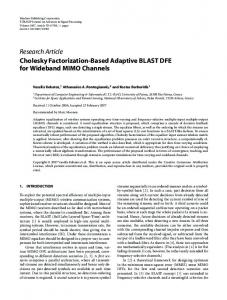
Figure 1.

Global Matrix of a 6x6, symmetric checksum matrix to be used in demonstration of algorithm.

II. A LGORITHM A. Algorithm Overview The algorithm functions by reserving an extra row and column of processors to hold a checksum of the values, which will be called the checksum row and column respectively. In this row and column of processors, a sum of the respective values of the other blocks in the same column and row, respectively, will be kept. As each block will contain MB*NB data points, this checksum will actually be a matrix of size MB*NB values. For simplicity, this paper will only cover the case where the processor grid, without the checksum row and column, is square P by P. Additionally, the blocking is assumed to be square. In other words MB equals NB. Finally, for ease of implementation, the matrix is assumed to be evenly divisible into blocks, i.e. the modulus of N by NB is zero. While these assumptions greatly ease the implementation, this method can still be used for Cholesky factorizations where these conditions do not hold. However, the demonstration of the extension of this method for other conditions will be contained in future work. The first step in the algorithm is to perform a checksum by two reductions of the values in each processor column and row into the checksum row and column respectively. The reduction can be done as first a row-wise sum reduction, and then a column-wise sum reduction. This means the reduction will actually be checksumming data from nonadjacent parts of the global matrix into the checksum matrix. However, as the checksum is in the respective positions of each local matrix, the overall global matrix checksum is preserved. Also note that this step needs to be performed whether a failure occurs or not, but it only occurs once per execution of the algorithm. The reduction can be done via either pipeline method or binomial tree method, depending on which is faster, based on the number of elements each process holds and the network parameters. With additional modification to the Cholesky low level block details, it would be possible to only use a checksum row without a checksum column. However, for ease

of implementation and as future work will require this extra column for two failure recovery, this algorithm will include both checksum row and column. The inclusion of the checksum column eases the implementation as the current ScaLAPACK Cholesky routine, PDPOTRF, requires a square, symmetric matrix. If only a checksum row were added, the matrix would no longer be square, and thus would no longer be symmetric. However, with the checksum row and column the matrix forms into a N+MXLLDA by N+MXLLDA matrix, where MXLLDA is the number of elements in one row or column of the submatrix stored on one processor. MXLLDA will be the same as NB only in the case that each processor holds only one block, as opposed to the widely used block cyclic techniques. Most of the time MXLLDA will be larger than NB. The execution of the Cholesky routine proceeds just as a normal blocked outer product routine would with the following exception: every P iterations, when a checksum block would be the next block to be used as the matrix diagonal, the algorithm will jump to the next iteration. As such, no additional iterations will be performed in the running of the Cholesky routine. However, each iteration may take longer due to the additional communication and time due to the existence of the checksum row and column. Other than this, the Cholesky routine functions as a standard block cyclic routine, such as is found in ScaLAPACK’s PDPOTRF. After any given iteration of the inline algorithm, the global matrix will contain three different parts. Figure 2 shows the breakdown of a matrix after one iteration. Specifically, in the inline algorithm, one part will consist of the partial result matrix L, the unfactorized part B, and data that is no longer used. The L portion of the matrix actually holds the partial result of the matrix L. This section is all in the lower triangle, and expands from its more filled columns to less filled columns. The second part is the B matrix, which contains the yet to be factorized part of the matrix. This is always a square section consisting of the lower right corner of the global matrix, from one column to the right of

Figure 2. Global Matrix of a 6x6 checksum matrix in a 4x4 processor grid after one iteration. The block size is 1. Green shows parts of L. Blue shows valid data in B. Red shows parts of B that are invalid. Orange shows n longer needed sections.

the end of L. In theory this is a symmetric matrix, though in ScaLAPACK the symmetry is not naturally maintained and need not be maintained for the algorithm to work. Specifically, this is because the division by the diagonal element through a row can be combined in a single loop with the updating of the b vector, which is the vector that is a precursor to the next column of L. As it is a symmetric matrix, the other half of the matrix can be used to calculate the L matrix as necessary, and therefore updating the upper triangle of B is not necessary. As such, the B matrix will not be symmetric for most of the execution. The rest of the matrix is no longer used. This is the remaining section of the matrix, which forms something that looks like the transpose of L minus the diagonal. A sample matrix is provided showing the progression of the matrix parts through three iterations, starting with the second iteration. The first iteration is often handled separately as additional checks are taken. As such, this is how ScaLAPACK’s routine is shown, and for convenience the second iteration is shown first. The row checksums are maintained differently based upon what section of the matrix they are in. For data that is in the L section of the matrix, the checksum is the sum of the entire column of corresponding local entries up until the diagonal. For data in the B section of the matrix, the checksum will be the sum of the elements in the column of the B matrix, including those past the diagonal. However, these elements must be of the true, symmetric B matrix rather than the undefined data that results from the ScaLAPACK routine. For data in the no longer used section of the matrix, no checksum is maintained and it need not be. If a piece of data is destroyed in this section, it can be ignored or set to zero. This view is valid from the standpoint of the global view of the matrix. However, in a block cyclic distribution, one processor may contain data from all three sections. Thus, upon a failure, each element must be examined individually to determine how it should be recovered. One common framework that eases the complexity of recovery is if the entire matrix is a state where checksums match up by the

respective elements of the column above them. The goal of this is simply to be able to do a reduction on the column to be able to recover the data. In order for this to work, elements of the unused section of data must be set to zero so as to have no effect, and the data of the checksum processors should be negated. In this formation, the result of a sum reduction will either be the values for the data if the processor that failed was a contained a checksum, or the negation of values for the data in all other cases. As a reduction is to be performed, this should not occur in the original matrix, but rather in a ’work’ matrix that will be used by the reduction call. When a failure occurs, the algorithm restores the values of the failed data to the failed processor. In order to do this, the following preconditions must be met: the row and column of the failed processor must be known, it must be assumed that no additional processors will fail during recovery, a copy of the most recent version matrix being operated on must be available where no items have been changed since the last recoverable point, and knowledge of what the last successful iteration of the Cholesky routine was. When a processor fails, due to the block cyclic nature of the data structure, it is possible for multiple blocks of data to need to be recovered from different parts of the matrix. However, they will all be held on processors that have either a process row or processes column that is the same as the process column of the failed processor. B. Transpose Method A stable method to compute the data lost due to failure is to perform a transpose of elements needed and then reduce column wise. The first step is to zero all elements that are above the diagonal in the process column of the failed processor. The next step is to make the B section symmetric for the column of the failed processor. This can be done through several methods. The na¨ive method is to copy the matrix, zero out all but the b section, take the transpose, zero the diagonal in the transpose, and then add the transpose back to the original matrix. Unfortunately, in ScaLAPACK taking the transpose of a matrix requires using PDGEMM.

Figure 3.

Status of global matrix after two step iterations of the Cholesky algorithm.

Figure 4.

Status of global matrix after three step iterations of the Cholesky algorithm.

if Local Node Failed then Data ← 0 end if if Above Diag AND Column = Failure Column then Receive(Data, Transpose) end if if Below Diag AND Row = Failure Column then Send(Data, Transpose) end if if Column = Failure Column then if Row = Checksum Row then ColumnReduce(F ailureRow, −Data) else ColumnReduce(F ailureRow, Data) end if end if Figure 5. The steps performed by each node to recover from a failure. Data is the local data matrix, Row is the processor row, Column is processor column, Failure Row and Column are the row and column of the failed node. Send, Receive, and ColumnReduce represent calling the MPI functions buffered appropriately for the size of data within the implied communicator.

The recovery method would be as computationally expensive as redoing the problem if it is necessary to transpose the whole matrix. Instead, it is possible to transpose only part

of the matrix, the B section, which makes for significant savings if the failure occurs later in the process. In a square matrix, with square blocks, in a square process grid, it is possible to transpose more easily by trading data between transposed processors in the process grid. While this seems like a straightforward method, one needs to consider that after the data is received it needs to be transposed within the cell and zeroed if it is not part of the B matrix going forward. This is shown in figure 8 and figure 9. This process is more complicated if the blocks are not square. III. I MPLEMENTATION In order to evaluate the method, two separate functions were compared for doing the Cholesky factorization. The first, PDPOTRF, is the ScaLAPACK function for doing Cholesky factorization. In order to simulate a failure, a second Cholesky factorization routine was written that assumes the full matrix with checksum row and column are given as parameters. During this method, it skips any data blocks along the diagonal that belong to the checksum processes. At the end of the method, the contents of the first P-1 by P-1 processor contents are examined to verify they match the result from a standard call to PDPOTRF on the matrix without the checksum processes. To verify correctness, small scale tests were run and the sum of squared error of original

Figure 6. A checksum matrix in the transpose method with block size of 2, yellow and white. The yellow and white has been left on the horizontal row to show that the data has come from the transpose. In general, it is easier and not much more costly to transpose the entire B matrix as opposed to just the failed processor column.

Figure 7.

The local view of the global matrix shown in figure 6.

matrix values versus recovered matrix values was calculated. For matrices on the order of ten by ten or less, the residual was on the order 10−30 . Unfortunately, verifying accuracy in this manner does not scale well as the size of the matrix increases. For the larger tests, comparing the one norm of the residual divided by the one norm of the original matrix, the recovery routine was verified to be accurate and scalable. This method has three additional parameters that specify where and when a failure occurs. Specifically, it takes the row and column of the process to fail and the iteration failure will occur. There are weaknesses to this simulation approach, specifically that in a real recovery routine, it would be required to use the local copy of the matrix saved after every iteration. This is also not adequate to do a full scale simulation assuming an exponential distribution of failure. However, it successfully tests that the recovery method works and the time required to recover by this method. The recovery function has two phases. In the first phase it sets up the checksum recovery so as to make a column reduction to the failed processor provide all the data needed to recover. In the second phase, the actual reduction occurs and the failed processor uses the data to reset its values in the global matrix. The first phase requires that each processor go through

its elements and determine which will be necessary for recovery. In the end, this will be maintained in a temporary matrix, which will in turn be used to perform the reduction. Improvements in the future might include looking at multiple reductions for individual segments of data to be communicated rather than analyzing the whole local matrix. However, for now, the local matrix is analyzed and separated as follows. In the first step, all matrix elements that are in the upper triangle of the global matrix are set to zero in the temporary matrix, and the ones in the lower triangle are copied into the temporary matrix. The checksum columns are copied in as the negation of their value in the original matrix. The negation is stored such that with a summation reduction call, the value in the failed process will be the negation of the value it should recover to without having to do a second reduction against the checksum row. In the case that it is a processor in the checksum row that has failed, then the value in the failed process after the reduction is complete will be the value it should have, and not its negation. In the inline blocked version of the Cholesky factorization, the L matrix expands by NB columns with each iteration, and subsequently the B matrix shrinks by NB columns (and thus NB rows as well since it is square). Keeping track of the current section of the matrix that is in B versus L is vital,

Figure 8. The overall block ownership by processor in the global grid for the earlier figures. Each color represents a processor and each square represents a block that belongs to the processor which it is colored. The labeled blocks show an example that each processor will only communicate at most with one other processor when all is square. For those on the diagonal, it can be seen that they only communicate with them self, either on the diagonal, or from one corner to another.

Figure 9. The actual blocks for the processors shown from the example. The labeled numbers correspond to the labeled blocks in the earlier figure. The communicated data will have to be transposed block wise to fill the invalid data with valid data. Also, note that each processor must both send and receive data, though one has more valid data to send than the other.

as the remainder should be ignored or zeroed. Additionally, since the B section of the matrix is not symmetric in ScaLAPACK, it is first necessary to get the transpose of this section of the matrix, find its transpose (minus the diagonal), and add it back to the temporary matrix. In the second stage, a column-wise by process grid communicator is established. If the column contains the failed process, then a summation reduction is performed. At this point the result matrix is retasked for the purpose of storing the reduction result. The value in the reduction result then needs to be processed and put into the original matrix. In the case that the failed process is in the checksum row, no processing is necessary and it can be simply be copied in. If it is any other row, as discussed before, the negation of the value in the result matrix must be put into the original matrix. Upon completion of this step, the original matrix is recovered.

on the evaluation of the algorithm. Each processor held a local sub-matrix with 5000 by 5000 elements, using blocking of 100 by 100. The initial symmetric positive definite matrix was created by constructing a matrix on a sub-grid of size P1 by P-1 containing pseudo random double precision values between zero and one, and then multiplying the transpose of that matrix against itself. Thus, the initial matrix for the 4 by 4 grid would have a process grid of 3 by 3, and a total size of 15000 by 15000 double precision elements. This matrix size was selected as it resulted in a maximum memory utilization by node of about 80 percent. A sample memory utilization graph is presented in figure 10.

IV. E VALUATION The implementation was tested on square process grids with process grid sides, P, of 4, 5, 6, 7, and 8. The processors exist on nodes with 8 processors per node. The processors are 2.66 GHz with 16GB of memory shared by the processors on each node. As not all grid sizes fit evenly on processors, the processors were selected so as to minimize the number of nodes required. The work was done on a dedicated cluster environment for high performance computing so as to minimize the impact of other processes

Figure 10.

Memory usage on single node from execution beginning.

The program run consisted of a test of twenty runs of FTPDPOTRF on the full matrix and twenty runs of PDPOTRF on the initial matrix. In the case of the FTPDPOTRF runs, one failure was simulated on each run and

a small fraction of the processing of the routine in general. Thus, while it does contribute to the initial overhead, it does not change order of the overall execution time. Depending on the matrix and network characteristics, this could be improved using a different reduce function implementation.

Figure 11.

Memory usage on single node showing execution finish.

the time taken in the recovery routine was captured. As there was additional time required to capture the failure time and verify the result, the total time for FTPDPOTRF was exaggerated and thus the recovery time will be estimated by the direct time for the recovery rather than the difference between the whole run and that of PDPOTRF. However, the overhead was calculated on these values regardless to show a worst case comparison. In all programs, the first run was discarded as the startup time was highly variable, leaving results on the remaining nineteen. The result of the runs by processor were averaged, as is noted on figure 15. The 90 percent confidence intervals shown were calculated assuming a normal distribution as it is estimating a mean with several samples. The results suggest that the execution of the FTPDPOTRF are slower, but on the same order of time required to perform the standard function PDPOTRF for the initial matrix.

Figure 12. Size

Trend for Time for Initial Checksum vs. Process Grid Side

Another question of overhead relates to the generation of the checksum in the checksum row and column. In this algorithm, this operation only needs to be performed once and requires two reduce calls. A sample time by process size to do this checksum using the default MPI Reduce function is shown in figure 12. As can be seen, this amount is increasing relative to the process grid size, but only requires

Figure 13. Size

Average Recovery Time in Algorithm vs. Process Grid Side

An additional concern was the time required to recover from a failure. Figure 13 shows the recovery times based on process grid side size for FTPDPOTRF. Since the recovery time is much less than the time to re-perform the entire function, this method indeed shows promise to improve expected execution times. It should be noted that the sum of all the additional overhead does not quite equal the difference in running time between FTPDPOTRF and PDPOTRF in figure 15. This is due to additional result validation steps that explore the accuracy of the recovery algorithm when a failure occurs, but for actual use this validation should be removed. Regardless, even with this additional validation, FTPDPOTRF is on the same order as PDPOTRF. As the time spent in overhead is increasing linearly while the algorithm is increasing more than quadratically, the overhead as a percent of total runtime is trending to reduce as the matrix grows, as can begin to be seen in figure 14. The accuracy of the recovery routine was verified by comparing the resulting matrix with a copy of the matrix saved before the fault is simulated. During the simulation of the fault, all entries in the local submatrix of the simulated failed processor are set to zero. After the routine completes, the one norm of the residual was taken and divided by the one norm of the initial matrix. For all process grid sizes, this value was much less than one and decreasing as shown in table I. As such, this is a sign that the method is numerically stable, though future tests with increasing scales will continue to be monitored to verify this. Additionally, an element by element comparison was done on a small scale problem to verify the accuracy.

Figure 14. Trend of Average Overhead as a Fraction of Total Function Runtime vs. Process Grid Side Size

recovery algorithm is significantly smaller than the time to re-perform the entire factorization. Furthermore, as the recovery algorithm never accesses more than a constant factor of processors in respect to the process grid side size, the recovery time should not grow as fast as the process grid. Future research will explore a full analytical approach to the analysis of the runtime of this algorithm to verify this. Additional research will also study the effect of process grid size on the overhead and recovery time of this algorithm. Another avenue to be explored will be to simulate a more appropriate failure model, such as an assumption of a constant failure rate. The performance could then be compared to the expected to existing diskless checkpointing schemes and previous algorithmic approaches to ascertain under what parameters each performs best. Another potential area of research is the development of this method for multiple failures, as other research demonstrates is possible. Expanding this technique to QR and other commonly used factorizations needs to be researched. Finally, as this has already been implemented for ScaLAPACK for certain ideal circumstances, development of a more robust implementation as well as use of MPI implementations with fault tolerant capabilities should be utilized to form a functioning system. ACKNOWLEDGMENT The authors would like to thank the anonymous peer reviewers for their suggestions that aided in improving this paper.

Figure 15. Average Total Runtime of FTPDPOTRF (on P by P) compared with PDPOTRF (on P-1 by P-1) vs. Process Grid Side Size (P)

V. C ONCLUSION The results indicate that this method of algorithmic recovery executes on the same order as the existing nonfault tolerant PDPOTRF. The overhead scales well in that it will grow linearly in relation to the size of the side of the process grid, whereas the process grid grows quadratically. Thus, the overhead will reduce with respect to execution time for increasing process grid sizes. The runtime of the Process Grid Side 4 5 6 7 8

Accuracy 0.164 0.031 0.020 0.014 0.010

Table I N ORM OF RESIDUAL MATRIX AFTER RECOVERY DIVIDED BY NORM OF ORIGINAL MATRIX .

R EFERENCES [1] A. A. Al-Yamani, N. Oh, and E. J. McCluskey, “Performance evaluation of checksum-based abft,” Defect and FaultTolerance in VLSI Systems, IEEE International Symposium on, vol. 0, p. 0461, 2001. [2] J. Anfinson and F. T. Luk, “A linear algebraic model of algorithm-based fault tolerance,” IEEE Trans. Comput., vol. 37, no. 12, pp. 1599–1604, 1988. [3] R. Banerjee and J. A. Abraham, “Bounds on algorithm-based fault tolerance in multiple processor systems,” IEEE Trans. Comput., vol. 35, no. 4, pp. 296–306, 1986. [4] P. Banerjee, J. T. Rahmeh, C. Stunkel, V. S. Nair, K. Roy, V. Balasubramanian, and J. A. Abraham, “Algorithm-based fault tolerance on a hypercube multiprocessor,” IEEE Trans. Comput., vol. 39, no. 9, pp. 1132–1145, 1990. [5] G. Bosilca, R. Delmas, J. Dongarra, and J. Langou, “Algorithm-based fault tolerance applied to high performance computing,” Journal of Parallel and Distributed Computing, vol. 69, no. 4, pp. 410 – 416, 2009. [Online]. Available: http://www.sciencedirect.com/science/article/B6WKJ4V8GB44-2/2/2658d9756341bece20e06d1485456678

[6] Z. Chen and J. Dongarra, “Algorithm-based checkpoint-free fault tolerance for parallel matrix computations on volatile resources,” Parallel and Distributed Processing Symposium, International, vol. 0, p. 76, 2006. [7] Z. Chen and J. Dongarra, “Algorithm-based fault tolerance for fail-stop failures,” IEEE Transactions on Parallel and Distributed Systems, vol. 19, no. 12, pp. 1628–1641, 2008. [8] Z. Chen, “Optimal real number codes for fault tolerant matrix operations.” in Proceedings of the ACM/IEEE SC09 Conference. ACM Press, 2009.

[13] D. Hakkarinen and Z. Chen, “N-level diskless checkpointing,” High Performance Computing and Communications, 10th IEEE International Conference on, vol. 0, pp. 384–391, 2009. [14] K.-H. Huang and J. A. Abraham, “Algorithm-based fault tolerance for matrix operations,” IEEE Transactions on Computers, vol. C-33, no. 6, pp. 518–528, June 1984. [Online]. Available: http://dx.doi.org/10.1109/TC.1984.1676475 [15] Y. Kim, J. S. Plank, and J. Dongarra, “Fault tolerant matrix operations using checksum and reverse computation,” in 6th Symposium on the Frontiers of Massively Parallel Computation, Annapolis, MD, October 1996, pp. 70–77.

[9] J. Choi, J. J. Dongarra, L. S. Ostrouchov, A. P. Petitet, D. W. Walker, and R. C. Whaley, “Design and implementation of the scalapack lu, qr, and cholesky factorization routines,” Sci. Program., vol. 5, no. 3, pp. 173–184, 1996.

[16] J. Plank, K. Li, and M. Puening, “Diskless checkpointing,” Parallel and Distributed Systems, IEEE Transactions on, vol. 9, no. 10, pp. 972–986, Oct 1998.

[10] E. N. Elnozahy and J. S. Plank, “Checkpointing for peta-scale systems: A look into the future of practical rollback-recovery,” IEEE Trans. Dependable Secur. Comput., vol. 1, no. 2, pp. 97–108, 2004

[17] D. Tao, C. Hartmann, and Y. S. S. Han, “New encoding/decoding methods for designing fault-tolerant matrix operations,” IEEE Transactions on Parallel and Distributed Systems, vol. 7, no. 9, pp. 931–938, 1996.

[11] G. E. Fagg, E. Gabriel, Z. Chen, T. Angskun, G. Bosilca, J. Pjesivac-grbovic, and J. J. Dongarra, “Process fault tolerance: semantics, design and applications for high performance computing,” in International Journal for High Performance Applications and Supercomputing, 2004, p. 2005.

[18] L. N. Trefethen and D. Bau, Numerical Linear Algebra. SIAM: Society for Industrial and Applied Mathematics, June 1997. [Online]. Available: http://www.amazon.com/exec/obidos/redirect?tag=citeulike0720&path=ASIN/0898713617

[12] E. Gabriel, G. E. Fagg, G. Bosilca, T. Angskun, J. J. Dongarra, J. M. Squyres, V. Sahay, P. Kambadur, B. Barrett, A. Lumsdaine, R. H. Castain, D. J. Daniel, R. L. Graham, and T. S. Woodall, “Open mpi: Goals, concept, and design of a next generation mpi implementation,” in In Proceedings, 11th European PVM/MPI Users Group Meeting, 2004, pp. 97–104.

[19] N. H. Vaidya, “A case for two-level distributed recovery schemes,” in In ACM SIGMETRICS Conference on Measurement and Modeling of Computer Systems, 1995, pp. 64–73. [20] N. H. Vaidya, “Another two-level failure recovery scheme,” College Station, TX, USA, Tech. Rep., 1994.