Hindawi Publishing Corporation Mathematical Problems in Engineering Volume 2013, Article ID 601482, 11 pages http://dx.doi.org/10.1155/2013/601482
Research Article Circular Orbit Target Capture Using Space Tether-Net System Guang Zhai, Jing-rui Zhang, and Zhang Yao School of Aerospace Engineering, Beijing Institute of Technology, Beijing 100081, China Correspondence should be addressed to Guang Zhai;
[email protected] Received 1 November 2012; Revised 16 February 2013; Accepted 5 March 2013 Academic Editor: Tadashi Yokoyama Copyright © 2013 Guang Zhai et al. This is an open access article distributed under the Creative Commons Attribution License, which permits unrestricted use, distribution, and reproduction in any medium, provided the original work is properly cited. The space tether-net system for on-orbit capture is proposed in this paper. In order to research the dynamic behaviors during system deployment, both free and nonfree deployment dynamics in circular orbit are developed; the system motion with respect to Local Vertical and Local Horizontal frame is also researched with analysis and simulation. The results show that in the case of free deployment, the capture net follows curve trajectories due to the relative orbit dynamic perturbation, and the initial deployment velocities are planned by state transformation equations for static and floating target captures; in the case of non-free deployment, the system undergoes an altitude libration along the Local Vertical, and the analytical solutions that describe the attitude libration are obtained by using variable separation and integration. Finally, the dynamics of postdeployment system is also proved marginally stable if the critical initial conditions are satisfied.
1. Introduction In the last two decades, space robotic systems for on-orbit capture have received significant attention. Some of these space robotic systems are used for orbital debris capture and removal. Among the proposed robotic systems, the capture tools are usually designed with rigid facilities, such as robotic manipulators and latch structures [1–3]. Although the rigid capture tools have been successfully validated in some space robotic missions, the safety challenges still exist when they are used for noncooperative target capture [4–6]. In order to deal with noncooperative space target capture, the flexible tether-net system (TNS) is proposed in this paper. Compared with rigid capture robotic system, TNSs have more potential advantages including enhanced error tolerance, increased capturing range, and reliable safety. In ESA (Europe Space Agency), TNS has been proposed as the on-orbit capture robotic system named “ROGER” [7–9], and this system will be used to capture and re-orbit the nonfunctional geostationary satellites in the future. Tremendous challenges ranging from dynamics to control are involved when TNS is used for on-orbit capture, and one predominant challenge is to obtain an insight into the deployment dynamics of the system, which is critical to ensure accurate and safety captures [10–12]. Generally
speaking, TNS can be deployed with connecting tether slack or tightened, and naturally the deployment dynamics, comprehensively governing the relative motion between the capture net and target, can be treated as a combination of relative dynamics and attitude dynamics. The relative dynamics, expediently presented by second-order linear equations, describes the target motion with respect to Local Vertical Local Horizontal frame. The attitude dynamics mainly illustrates the in-plan and out-of-plan librations during deployment and station keeping. Tethered satellite system (TSS) has attracted considerable attention in the past decades; numerous researches have researched the different aspects of TSS dynamics, especially motion analysis for deployment, station keeping, and retrieval. Typical TSS is comprised of two satellites connected with tether moving in central gravitational field. Kane made very basic dynamic research and analysis of TSS [13]. With mass less tether assumption, Yu et al. have studied the two-dimensional dynamics of TSS [14]. Fujii and Ichiki studied the nonlinear dynamic behaviors of tethered subsatellite in the station keeping phase [15]. Takeichi et al. obtained the periodic solutions for TSS in an elliptical orbit [16]. Furthermore, many researchers have developed control strategies for TTS deployment and station keeping. Details of other achievements can be obtained from the cited references [17–23].
2 Other conceptual applications of tethered space system, such as orbital transportation and momentum-exchange [24], have been researched recently. Rather than the ordinary TSS, this type of tethered system is generally librating or spinning with prescribed rotation in orbital frame, and the tools on the tether tip capture the payload only when it rendezvouses with target; therefore, series of papers have focused on the libration and spinning control problem in order to enable precise rendezvous and captures. Tethermediated orbital rendezvous was firstly mentioned by Carroll [25]; after that Stuart [26] designed a single tether system to perform the in-plan capture. The predictive controller was developed for the libration regulation and damping. Blanksby and Trivailo [27] developed tether crawler system for the orbital transportation, and a corresponding controller based on length modulation was used. Williams developed nonlinear optimal controller and receding horizon controller for the elastic tether system. Besides circular orbit, Williams [10, 11, 20] also studied the capture of in-cooperative payload in elliptic orbits. Although series of control strategies have been proved effective, though numerical simulations, spinning tethered system is still far from practical employment. Actually all of the control strategies are developed with various simplifications, which means that when those controllers are used, spinning tethered system will be affected by the nonlinearity and coupling, time-delay, and environmental disturbance, and therefore it is extremely difficult for the controllers to precisely offer a position and velocity match between tether tip and target, which is even worse for the long tether system. However, the TNS proposed in this paper is significantly different from the typical space tethers in the following aspects; firstly, the capturing net of TNS can be deployed with the connecting tether slack, while this is not allowed for typical space tethered system; secondly, the TNS is proposed to deploy rapidly in the orbit, which means that the marginal dynamics stability for typical space tethered can hardly be sustained in the case of TNS deployment; thirdly it is assumed that the tether length of TNS is several hundred meters, so the whole capture operation probably only takes several seconds and the long-term disturbance, for example, J2 gravitational perturbation and atmospheric drag force, can be almost neglected; finally, the dynamic parameters of TNS will be changed instantly after the target is captured. Due to the above reasons, it is necessary to establish the TNS deployment dynamics according to the system characteristics if successful captures are expected. This paper will focus the research on the deployment dynamics of TNS system; the whole paper is organized as follows: in Sections 2 and 3, the free deployment dynamics is developed with respect to Local Vertical Local Horizontal frame; then the relative motion between the capture net and target is formulated with state transformation equations; deployment velocity planning method for static and floating target capture is also obtained based on state transformation equations. In Sections 4 and 5, the non-free deployment dynamics is developed with Lagrange theorem; after that the in-plan motion is decoupled from the out-of-plan motion, and the analytical solution for in-plan libration is obtained
Mathematical Problems in Engineering Target
𝜌nt
Capture net
𝜌𝑡 𝜌𝑛
𝑅𝑖
𝑅𝑡
𝑌𝑜
𝑋𝑒
𝑍𝑏
𝑋𝑏 𝑅
𝑍𝑜 𝑌𝑏 Platform
𝑋𝑜
Earth 𝑍𝑒
𝑂𝑒
𝑌𝑒
𝜔
Figure 1: Reference frame for freedeployment dynamics modeling.
with variable separation. At last the dynamics behaviors of post-deployment system are also studied.
2. Free Deployment Dynamics Free deployment means connecting tether retains slack when capturing net is released towards the target. In this case, there is no external force acting on the capturing net other than gravitational force, and then the dynamic coupling between the capturing net and platform can be almost ignored. Now we consider that the space tether net system is in a circular orbit, and the target spacecraft is flying in a near circular orbit with small eccentricity; the platform, capturing net, and target are treated as a mass point, so we can assume that the target spacecraft is close enough to the tether net system when the capturing net is released. As Figure 1 shows, two reference frames, Earth Inertial (EI) frame and Local Vertical Local Horizontal frame, are defined, respectively, for developing the deployment dynamics. The Earth Inertial frame is a nonrotating frame with its origin point located at the mass centre of the earth; its 𝑥axis and 𝑧-axis are aligned with the equinox and spin axis of the earth, respectively. The Local Vertical Local Horizontal (LVLH) frame, also named orbital frame, is a rotating frame. Its origin point is located at the mass centre of the tether net system. The 𝑥-axis is aligned with vector from the Earth’s centre of mass to the spacecraft centre of mass, and 𝑧-axis is aligned with the orbital velocity vector of the tether net system. Based on Newton’s law, the dynamics of mass point in the EI frame can be expressed as follows: 𝜇R R̈ 𝑖 = 3𝑖 + f𝑑𝑖 + 𝑢𝑑 , 𝑅𝑖
(1)
where R𝑖 denotes position vectors of capturing net and target spacecraft with respect to the Earth Inertial frame, 𝜇 is the Earth gravitational coefficient with constant value, f𝑑𝑖 denotes
Mathematical Problems in Engineering
3
perturbations such as sun pressure and earth oblateness, and 𝑢𝑑 represents control force acting on the centre of mass. Since the capture operation is performed within a short-time interval, the long-term external perturbations can be ignored reasonably, and then both the system and target spacecraft can be considered moving in Keplerian orbits. The main goal of the free deployment dynamics is to interpret the relative motion between the capture net and target; therefore, based on (1), we can obtain the relative model by the following vector propagation: 𝜌̈ 𝑒𝑖 =
𝜇R𝑖 𝜇R𝑗 − 3 . 𝑅𝑖3 𝑅𝑗
(2)
In the above equation, 𝜌𝑒𝑖 denotes the position vectors of the target or capturing net in the orbital frame and the superscript 𝑒 denotes the relative acceleration and the position represented in EI frame. The relative dynamics is formulated by a second-order nonlinear equation. However, (2) cannot be used in practice since the position vectors R𝑖 can not be acquired directly with the on-board relative sensors. Therefore, according to the vector transformation principle between rotating and inertial frame, the dynamic equations can be formulated with vectors expressed in LVLH frame alternatively, and then we have 𝜌̈ 𝑜𝑖 = 𝜌̈ 𝑒𝑖 − 2𝜔 × 𝜌̇ 𝑜𝑖 − 𝜔 × (𝜔 × 𝜌𝑜𝑖 ) − 𝜔̇ × 𝜌𝑜𝑖 ,
(3)
where 𝜔 is the orbital angular velocity of tether net system and the superscript 𝑒denotes the vectors expressed in EI frame. Now define the vector 𝜌𝑜𝑡 = [𝑥𝑖 , 𝑦𝑖 , 𝑧𝑖 ]𝑇 and accordingly, when expressed in LVLH frame we have R = [0, 0, 𝑟]𝑇 , R𝑡 = [𝑥𝑖 , 𝑦𝑖 , 𝑟 + 𝑧𝑖 ]𝑇 , where 𝑟 is semimajor axis of tether net system, substituting R and R𝑡 into (2), then expanding the right side of the formulation with Taylor series; through second-order approximation, 𝜌̈ 𝑒𝑖 can be rewritten as follows: 𝜌̈ 𝑒𝑖 = 𝜔𝑇 𝜔 (R − (1 +
3𝑦𝑡 ) ⋅ R𝑡 ) . 𝑟
(4)
Substitute (4) into (3), then we can get target or capture net motion equations in LVLH frame by using (3); the relative acceleration between the capturing net and target expressed in LVLH frame can be represented as follows: 𝜌̈ 𝑜𝑛𝑡 = 𝜌̈ 𝑒𝑛𝑡 − 2𝜔 × 𝜌̇ 𝑜𝑛𝑡 − 𝜔 × (𝜔 × 𝜌𝑜𝑛𝑡 ) ,
(5)
3. Free Deployment Simulation and Analysis 3.1. Free Deployment Planning. The relative motion of capturing net after deployment is described with (6). Obviously the capturing net and target should locate at the same position on specific time if successful capture is expected, which means 𝜌𝑜𝑛𝑡 = 0 after the specific time interval. Since most targets are floating unpredictably in orbital frame due to external perturbations, when tracking the target, synchronous regulation of deployment velocity is required consequently to ensure precise captures. Based on (6), the analytical solution of deployment dynamics can be rewritten with state transformation equations as follows: 𝜌 (𝑡) Φ (𝑡, 𝑡0 ) Φ12 (𝑡, 𝑡0 ) 𝜌 (𝑡0 ) ]( ) + 𝐵𝑢 (𝑡) . (7) ( ) = [ 11 𝜌̇ (𝑡) Φ21 (𝑡, 𝑡0 ) Φ22 (𝑡, 𝑡0 ) 𝜌̇ (𝑡0 ) Here, for short, we use 𝜌 to denote 𝜌𝑜𝑛𝑡 , 𝑡0 and 𝑡 denote the deployment time and capture time, obviously 𝜌 can be acquired with the relative sensors fixed on TNS, 𝐵 is input matrix with constant element, 𝑢(𝑡) is thruster force acting on the target during the deployment, the time expenditure, 𝑇 = 𝑡 − 𝑡0 , describes the time interval from the deployment beginning to the end, and it can be preset approximately according to deployment velocity and initial relative distance, Φ𝑖𝑗 (𝑡, 𝑡0 ) ∈ 𝑅3×3 is submatrix of state transformation matrix, and 𝜌(𝑡) = 01×3 when the target is captured, by defining 𝜃 = 𝜔(𝑡 − 𝑡0 ), 𝑆𝜃 = sin 𝜃, 𝐶𝜃 = cos 𝜃, then substituting these nomenclature into (7), and then the submatrix can be expressed, respectively, as follows: 1 0 6 (𝜃 − 𝑆𝜃 ) ], 0 Φ11 (𝑡, 𝑡0 ) = [0 𝐶𝜃 0 0 4 − 3𝐶 𝜃 ] [ 2 (1 − 𝐶𝜃 ) 4𝑆𝜃 − 3𝜃 0 ] [ 𝜔 𝜔 ] [ 𝑆𝜃 ] [ Φ12 (𝑡, 𝑡0 ) = [ 0 0 ], ] [ 𝜔 ] [ 2 (1 − 𝐶 ) 𝑆𝜃 𝜃 − 0 ] [ 𝜔 𝜔
(8)
0 0 6𝜔 (1 − 𝐶𝜃 ) ], 0 Φ21 (𝑡, 𝑡0 ) = [0 −𝜔𝑆𝜃 0 0 3𝜔𝐶 𝜃 [ ]
where 𝜌𝑜𝑛𝑡 represents the relative vector between capturing net
4𝐶𝜃 − 3 0 2𝑆𝜃 𝐶𝜃 0 ] . Φ22 (𝑡, 𝑡0 ) = [ 0 0 𝐶𝜃 ] −2𝑆 𝜃 [
𝜔𝜌̇ 𝑜𝑛𝑡 − 𝐾𝜔𝑇 𝜔𝜌𝑜𝑛𝑡 . 𝜌̈ 𝑜𝑛𝑡 = 2̃
Now supposing no relative maneuver was performed when the capturing net is approaching to the target, which is 𝑢(𝑡) = 0, then substituting the submatrix into (7), the ̇ can be calculated as follows when the ̇ 0 ) and 𝜌(𝑡) vectors 𝜌(𝑡 transformation matrix Φ12 (𝑡, 𝑡0 ) is nonsingular:
and target, and superscript 𝑜 denotes the vector described in LVLH frame. Furthermore, substituting (4) into (5), finally (5) can be simplified as follows: (6)
Equation (6) is a second-order linear equation, where 𝐾 is the coefficient matrix depending on-orbital angular ̃ denotes the skew matrix of orbital angular velocity, and 𝜔 velocity, and this equation mathematically illustrates the relative motion between the capturing net and target after the system deployment.
𝜌̇ (𝑡0 ) = −Φ−1 12 (𝑡, 𝑡0 ) Φ11 (𝑡, 𝑡0 ) 𝜌 (𝑡0 ) , 𝜌̇ (𝑡) = [Φ21 (𝑡, 𝑡0 )−Φ22 (𝑡, 𝑡0 ) Φ−1 12 (𝑡, 𝑡0 ) Φ11 (𝑡, 𝑡0 )] 𝜌 (𝑡0 ) . (9)
4
Mathematical Problems in Engineering Target type: floating Target states: [0, 0, 200], [0, 0.1, 0] Time expenditure: 40 seconds
Target type: static Target states: [100, 0, 0], [0, 0, 0] Time expenditure: 20 seconds 0
Capture position
0 −0.1
−100
−0.2
𝑧 (m)
𝑧 (m)
Capture net
−50
−0.3
−150 Floating target
−200
−0.4 −0.5 1
100 0.5
0 𝑦 (m)
−0.5
−1 0
−250 4
50 ) 𝑥 (m
Capture position 2 𝑦 (m 0 −2 )
(a)
−1
0
1
𝑥 (m)
(b)
Figure 2: Capture simulation for static targets and floating targets.
Equation (9) implies that if the time expenditure 𝑇 is given, both the initial and the final relative velocities are determined by the initial relative position; moreover, after ̇ 0 ) is obtained, we can get the deployment velocity of the 𝜌(𝑡 capture net as follows: 𝜌̇ 𝑛 (𝑡0 ) = 𝜌̇ 𝑡 (𝑡0 ) − 𝜌̇ (𝑡0 ) ,
(10)
where 𝜌̇ 𝑛 (𝑡0 ) is the initial deployment velocity, which is necessary for precise capture and 𝜌̇ 𝑡 (𝑡0 ) is the target initial velocity relative to the LVLH frame, and it can be acquired by the relative sensors on the platform. 3.2. Free Deployment Simulations. Series of capture simulations have been carried out to demonstrate the interrelationship among the deployment velocities, time expenditure, and initial states of target. Typically the targets have been classified into two groups: the first group consists of static targets located at V-bar of LVLH frame, while the second group consists of free floating targets. All the captures take place in the circular orbit of 600 km high altitude, and the capture simulations are completed with the connecting tether slacked. All the initial deployment velocities can be obtained by using (9) and (10). As shown in Table 1, the static target captures are simulated with time expenditures of 20 and 40 seconds, respectively, and corresponding targets locate in V-bar with zero initial velocity but different relative distances ranging from 100 m to 300 m; it should be noted that in the case the targets experience self-station keeping with respect to the original point of the orbital frame, which can be proved with (9). The same with static target captures, the floating target captures are also simulated with 20 and 40 seconds time expenditures, whereas their initial position is supposed on R-bar and Vbar with nonzero initial velocities. From the results we can see that for the static target captures, the 𝑧-components of release velocity are increased with the rising of capture distance, while the 𝑦-component velocities remain zero. For the floating target captures, an 𝑦-components velocity
Table 1: Parameters of free deployment capture simulations. Target type
Time expenditure (s) 20
Static 40
Floating
20 40
Targets states (m, m/s)
Release velocity (m/s)
[100, 0, 0], [0, 0, 0] [200, 0, 0], [0, 0, 0] [150, 0, 0], [0, 0, 0] [300, 0, 0], [0, 0, 0]
[4.99, 0, −0.09] [9.98, 0, −0.19] [3.75, 0, −0.14] [7.49, 0, −0.29]
[100, 0, 0], [0, 0.1, 0.1] [4.99, 0.10, −0.09] [0, 0, 200], [0, 0.1, 0] [0.20, 0.10, 10.02] [100, 0, 0], [0, 0.1, 0.1] [2.49, 0.10, 0.01]
equivalent to its initial component is needed for precise captures, which implies the fact that the 𝑦-directional motion is decoupled form the 𝑥 and 𝑧 directional motions. Figure 2 describes the motion trajectories of the capture net and floating targets in orbital frame; for the static target capture, the curvilinear trajectory is restricted in the orbital plan, while for the floating target capture, the curvilinear trajectory undergoes synchronous oscillation out of orbital plan.
4. Nonfree Deployment Dynamics 4.1. Reference Frames. A distinct characteristic of nonfree deployment is that the connecting tether keeps tightened when the capture net is deployed; the drag force acting on the capturing net differentiates its capture dynamics significantly from the Free-Deployment ones, and therefore the dynamics we developed in Section 2 can not be used here. The purpose of this section is to establish the nonfree deployment dynamics with a consideration of length alteration during the system deployment, and the in-plan and outof-plan liberations, which significantly impact the motions of
Mathematical Problems in Engineering
5
Target
Capture net
𝑌𝑜 𝑍𝑏 𝑌𝑜
𝑍𝑏
𝑋𝑒
𝑌𝑏 𝑙1
𝑋𝑏 𝑂𝑒
𝑍𝑜 𝑌𝑏
Earth 𝑍𝑒
𝑂𝑒
𝑋𝑜
Platform
𝑙2
𝛼
𝑍𝑜 𝑌𝑒
𝑂𝑐
𝛽
𝜔
𝑋𝑏
(a)
𝑋𝑜
(b)
Figure 3: Reference frame for freedeployment dynamics modeling.
capturing net relative to the targets, will be researched based on the dynamics model. In general, the dynamics of tether net system is very complicated due to its flexibility and external perturbations. In order to simplify the researches, the only external force acting on the tether system is the Newtonian gravity force of the Earth. Other external perturbations, such as Sun pressure, aerodynamic drag force, and gravity from the sun and other planets, are considered negligible. Moreover, the system is assumed to be moving in a circular orbit, and the target also locates in the coplanar orbit. Both the capture net and the target are treated as particles of masses. The reference frames used to develop the system dynamics are Earth Inertial frame (EI), Local Vertical Local Horizontal Frame(LVLH), and Body-Fixed frame(BF). The EI frame and LVLH are defined as in Section 2. All the reference frames can be demonstrated in Figure 3. The BF frame, whose elements are principal axes of inertia, can be defined as follows: the basic vector 𝑧𝑏 is directed from the platform to the capture net, and the second basic vector 𝑦𝑏 is obtained as follows: 𝑧 × 𝑦𝑏 𝑦𝑏 = 𝑏 . 𝑧𝑏 × 𝑦𝑏
(11)
Then the final basic vector 𝑥𝑏 can be achieved with righthand principle. The original point of the BF frame is fixed on the mass centre of the system. The definition of BF frame can be illustrated as in Figure 3. As described in Figure 3, 𝛼 and 𝛽 represent the in-plan and out-of-plane libration angular, respectively. 4.2. System Energy Function. Lagrange principles enable us to derive the dynamics of the system mathematically. However, kinetic and potential energy of the tether-net system must be obtained before the use of Lagrange principle. The proposed tether net system involves two types of energy components:
kinetic energy and potential energy. When the capture net is released in the orbit, the system total kinetic energy can be calculated through scalar summation of three terms as follows: 𝑇 = 𝑇𝑜 + 𝑇𝑑 + 𝑇𝑟 ,
(12)
where 𝑇𝑜 and 𝑇𝑑 represent the kinetic energy terms due to orbital velocity and deployment rate, respectively, while 𝑇𝑟 represents the term associated with the system altitude motions relative to EI frame. All kinetic energy terms can be calculated as follows, respectively: 2 1 𝑇𝑜 = 𝑀 [𝑓̇ 𝑟2 + 𝑟2̇ ] , 2
𝑇𝑑 =
1 1 [(𝑚𝑙12 + [𝑀 − 𝜌 (𝑙∗ − 𝑙)] 𝑙22 ) + 𝜌 (𝑙13 + 𝑙23 )] 2 3 2
2
̇ cos2 𝛽] , × [𝛽̇ + (𝑓̇ + 𝛼)
(13)
2
𝑇𝑟 =
𝑙̇
1 2 {[(𝑚 + 𝜌𝑙1 ) [(𝑀 + 𝜌𝑙∗ ) − 𝜌𝑙] 2 2𝑀 2
2 1 + (𝑀 + 𝜌 (𝑙∗ − 𝑙)) ( 𝜌𝑙 + 𝑚) ]} . 2
In the above equations, 𝑀 is total mass of the system, while 𝑚 and 𝑀 are the mass of capture net and platform and 𝑟 and 𝑓 denote the semimajor axis and true anomaly of the orbit, for the circular orbit remains constant value. 𝑙∗ and 𝑙 denote the total length and the deployed length of the tether, 𝜌 represents the line density of the tether and 𝑙1 and 𝑙2 denote the vector of endpoint with respect to original point of LVLH frame.
6
Mathematical Problems in Engineering
In general, the potential energy in gravitational field is defined as follows: 𝑉 = −∫ 𝜇 𝑚
𝑑𝑚 . 𝑟
(14)
With Taylor expansion and high-order terms neglected, the potential energy term induced by connecting tether can also be obtained with the following format: 𝑉2 = −
Obviously the total potential energies are associated with total mass of the system. Therefore, with particle mass assumptions, the total potential energies can be calculated separately: 𝑉 = 𝑉1 + 𝑉2 + 𝑉𝑒 ,
(15)
where 𝑉1 and 𝑉2 are the components associated with mass of particles, while 𝑉𝑒 is the elastic potential energy due to the tether deformation. According to the potential energies definition, we have 𝑀 + 𝜌 (𝑙∗ − 𝑙) 𝑚 𝑉1 = −𝜇 − 𝜇 . r + l1 r + l2
(16)
Here ‖ ⋅ ‖ denotes the vector mold. According to the relationship of vectors in Figure 2, we have −1/2 −1 2 2 r + 𝑙1 = (𝑟 + 𝑙1 + 2𝑟𝑙1 cos 𝛽 cos 𝛼) , −1/2 −1 2 2 r + 𝑙2 = (𝑟 + 𝑙2 − 2𝑟𝑙2 cos 𝛽 cos 𝛼) .
(17)
−1 r + 𝜌1 𝑙 1 [1 − 1 cos 𝛼 cos 𝛽 + 𝑟 𝑟
1 (22) 𝑉𝑒 = 𝐸𝐴𝑙𝜉2 , 2 where 𝐸 is the elastic ratio, 𝐴 is the cross-sectional area, 𝑙 is the length of deployed tether without deformation, and 𝜉 is the strain coefficient. 4.3. Equations of Motion. Through the definition of the Lagrange principle, we can get 𝐿 = 𝑇 − 𝑉,
2 1 1 3 ∑𝑚 [𝑓̇ 𝑟2 + 𝑟2̇ ] + [ (𝑚𝑙12 + [𝑀 − 𝜌 (𝑙∗ − 𝑙)] 𝑙22 ) 2 𝑖=1 𝑖 2
1 + 𝜌 (𝑙13 + 𝑙23 )] 3 2
𝑙12 2𝑟2
(3cos2 𝛼 cos2 𝛽 − 1)] ,
𝑙2 𝜇𝑚 𝑙 [1− 1 cos 𝛼 cos 𝛽+ 12 (3cos2 𝛼 cos2 𝛽 −1)] 𝑟 𝑟 2𝑟 −
𝜇 [𝑀 + 𝜌 (𝑙∗ − 𝑙)] 𝑙 [1 + 2 cos 𝛼 cos 𝛽 𝑟 𝑟 +
𝑙22 (3cos2 𝛼 cos2 𝛽 − 1)] . 2𝑟2 (20)
2
𝑙̇
2𝑀
2
2 1 + [𝑀 + 𝜌 (𝑙∗ − 𝑙)] ( 𝜌𝑙 + 𝑚) } 2
+
𝑙2 𝜇𝑚 𝑙 [1− 1 cos 𝛼 cos 𝛽 + 12 (3cos2 𝛼 cos2 𝛽 − 1)] 𝑟 𝑟 2𝑟
+
𝜇 [𝑀 − 𝜌 (𝑙∗ − 𝑙)] 𝑙 [1 + 2 cos 𝛼 cos 𝛽 𝑟 𝑟
Furthermore, substituting (18) and (19) into (16), the potential energy associated with the particle mass can be obtained as follows: 𝑉1 = −
2
1 2 × {(𝑚 + 𝜌𝑙1 ) [𝑀 + 𝜌𝑙∗ − 𝜌𝑙] 2
−1 r + 𝜌2 𝑙2 𝑙 1 [1 + 2 cos 𝛼 cos 𝛽 + 22 (3cos2 𝛼 cos2 𝛽 − 1)] . 𝑟 𝑟 2𝑟 (19)
(23)
where 𝐿 denotes Lagrange function. By substituting the kinetic and potential energies into (23), we have
̇ cos2 𝛽] + × [𝛽̇ + (𝑓̇ + 𝛼)
(18)
=
𝑙2 𝑙3 𝜇𝜌 [1 + 2 cos 𝛼 cos 𝛽 + 22 (3cos2 𝛼 cos2 𝛽 − 1)] . 𝑟 2𝑟 6𝑟 (21)
Otherwise, when the connecting tether is treated as spring with nonviscous assumption, the elastic potential energy will be involved as
𝐿 =
By using Taylor expansion and ignoring the high-order terms of (17), the formulation of the vector mold can be simplified as
=
−
𝑙2 𝑙3 𝜇𝜌 [1 − 1 cos 𝛼 cos 𝛽 + 12 (3 co s2 𝛼 cos2 𝛽 − 1)] 𝑟 2𝑟 6𝑟
+
𝑙22 (3cos2 𝛼 cos2 𝛽−1)] 2𝑟2
+
𝑙2 𝑙3 𝜇𝜌 [1− 1 cos 𝛼 cos 𝛽 + 12 (3cos2 𝛼 cos2 𝛽 −1)] 𝑟 2𝑟 6𝑟
+
𝑙2 𝑙3 𝜇𝜌 [1+ 2 cos 𝛼 cos 𝛽 + 22 (3cos2 𝛼 cos2 𝛽 −1)] 𝑟 2𝑟 6𝑟
1 − 𝐸𝐴𝑙𝜉2 . 2 (24)
Mathematical Problems in Engineering
7
By ignoring the tether mass and elastic potential energy term, the motion equations of the system can be derived with Lagrange formulation: 𝑑 𝜕𝐿 𝜕𝐿 )− = 𝑄𝑗 , ( 𝑑𝑡 𝜕𝑞̇ 𝑗 𝜕𝑞𝑗
(25)
where 𝑞𝑗 is the generalized coordinate and 𝑄𝑗 is the generalized force according to the generalized coordinate. Substituting (24) into (25), then, respectively, defining the generalized force 𝑇(𝑡), 𝜏(𝑡), 𝛾(𝑡), eventually we can get the governing nonlinear, coupled ordinary differential equations of motion as follows: 2 𝜇 2 ̇ cos2 𝛽] 𝑙 − 3 𝑙 ̈ − [𝛽̇ + (𝑓̇ + 𝛼) 𝑟
𝑇 (𝑡) × (3cos 𝛼 cos 𝛽 − 1) 𝑙 = , 𝑀 2
2
2𝑙 ̇ ̇ ̇ 𝛽̇ + (𝑓̇ + 𝛼) 𝛼̈ − 2 tan 𝛽 (𝑓̇ + 𝛼) 𝑙 3𝜇 𝜏 (𝑡) , + 3 cos 𝛼 sin 𝛼 = 𝑟 𝑀𝑙2 cos2 𝛽 2 𝑙̇ ̇ cos 𝛽 sin 𝛽 𝛽̈ + 2𝛽̇ + (𝑓̇ + 𝛼) 𝑙
−
3𝜇 2 𝛾 (𝑡) cos 𝛼 cos 𝛽 sin 𝛽 = . 3 𝑟 𝑀𝑙2
(26)
(27)
(28)
right side, so the system will remain stationary along the outof-plan direction: 2 3𝜇 𝑙̇ ̇ − 3 cos2 𝛼) cos 𝛽 sin 𝛽 = 0. 𝛽̈ + 2 𝛽̇ + ((𝑓̇ + 𝛼) 𝑙 𝑟
Based on the above analysis, the in-plan dynamics can be decoupled from the out-of-plan dynamics and then the inplan deployment dynamics can be described as 𝜇 𝑇 (𝑡) (3cos2 𝛼 − 1)] 𝑙 = 𝑟3 𝑀 ̇ ̇ 3𝜇 −2𝑙 ̇ 2𝑙 𝑓 𝛼̈ + 𝛼̇ + 3 cos 𝛼 sin 𝛼 = 𝑙 𝑟 𝑙 when 𝛽̇ = 𝛽 = 0. 2
̇ + 𝑙 ̈ − [(𝑓̇ + 𝛼)
3𝜇 2𝑙 ̇ 𝑙̇ ̇ 3 cos 𝛼 sin 𝛼 = 2𝛽̇ tan 𝛽𝑓̇ − 𝑓.̇ ̈ (𝛽̇ tan 𝛽 − ) 𝛼+ 𝛼−2 𝑙 𝑟 𝑙 (29) Assuming the system works with zero initial condition while the deployment rate 𝑙 ̇ is nonzero, then the right side of (29) can be treated as a combination of two coupling torques, which associated with out-of-plan motion and tether deployment, respectively, acting along in-plan direction; naturally the coupling torques generate in-plan motion even if the initial state is zero. However, for (28), there are no coupling torques associated with in-plan libration or tether deployment rate on the
(31)
5. Nonfree Deployment and Postdeployment Simulations 5.1. In-Plan Deployment Motions. Now consider an in-plan deployment taking place in circular orbit; then the deployment motion can be researched based on (31). Supposing that the deployment rate is remained constant, then according to (31), the generalized force acting on the connecting tether can be calculated as follows: 𝑇 (𝑡) = −𝑀 [(𝜔 + 𝛼)̇ 2 + 𝜔2 (3cos2 𝛼 − 1)] (𝑙𝑐̇ 𝑡 + 𝑙0 ) ,
(32)
where 𝑙𝑐̇ denotes the constant deployment rate and 𝜔 denotes orbit angular velocity, and it can be achieved by
In the above equations, we have 𝑇(𝑡) < 0 since the tether is tightened all the time, and 𝑓̇ is constant in any circular orbit. 4.4. In-Plan and Out-of-Plan Dynamic Decoupling. Equations (26)–(28) indicate that both in-plan and out-of-plan motions are coupled with the tether deployment, which means that when released towards the target, the initial velocity vectors will be changed gradually under the attitude perturbation; thus the shape of tether-net system will present a libration, and the capture net will follow a curve trajectory when approaching to the target. Now let 𝜏(𝑡) = 0, 𝛾(𝑡) = 0, that is, no external torques acting on the system, and then transform (27) as
(30)
𝜔=√
𝜇 = 𝑓.̇ 𝑟3
(33)
In order to research the in-plan motions during the deployment, series of numerical simulations were carried out with different initial deployment rate. The in-plan motions, including the libration amplitude and velocities, are demonstrated in Figure 4; Figure 5 shows the shape of tether net system when deployed with initial velocities of 10 m/s and 8 m/s, Figure 6 illustrates the control force acted on tether when deployed with different initial velocities. From the results we can see that the in-plan angle will gradually increase with time elapse. In general, the capture operation could be accomplished within 20 seconds, so throughout the whole deployment, the in-plan angle amplitude will remain less than 1.5∘ , and the amplitude of in-plan angular velocities will increase rapidly after the capture net is released, but it will be kept on a relative stable level after 5 seconds. Substituting (33) into (31), the in-plan libration dynamic can be expressed as 𝛼̈ +
−2𝑙𝑐̇ 2𝑙𝑐̇ 𝛼̇ = 𝜔 − 3𝜔2 cos 𝛼 sin 𝛼. 𝑙 𝑙
(34)
In the above equation, 𝜔 ≪ 1 (for example, when the space tether net system works in a circular orbit of 600 km altitude high, 𝜔 ≈ 0.001 rad/s) and 𝛼 ≪ 1 (according to simulation result in Figure 4), and then
8
Mathematical Problems in Engineering 0
0
−0.4
Velocity (deg/s)
Amplitude (deg)
−0.2
−0.6
−0.02
−0.04
−0.8
−1
0
5
10
15
20
−0.06
0
5
10 Time (s)
Time (s) 8 m/s 10 m/s
2 m/s 5 m/s
2 m/s 5 m/s
15
20
8 m/s 10 m/s
(a)
(b)
Figure 4: The in-plan motion during nonfree deployment. 100
80
𝑣 = 10 m/s
80
𝑣 = 8 m/s
60
𝑧 (m)
𝑧 (m)
60 40
40
20 20
0 −1
0
−0.5
0
−0.8
−0.6
−0.4 𝑥 (m)
𝑥 (m) (a)
−0.2
0
(b)
Figure 5: The shape of the system during deployment.
the term 3𝜔2 cos 𝛼 sin 𝛼 can be ignored and and the in-plan libration dynamics can be simplified as follows: −2𝑙𝑐̇ 2𝑙𝑐̇ (35) 𝛼̇ = 𝜔. 𝑙 𝑙 Then by using variable separation, (35) can be rewritten as 𝛼̈ +
2𝑙 ̇ 𝑑𝑡 𝑑𝛼̇ =− 𝑐 . 𝜔 + 𝛼̇ 𝑙0 + 𝑙𝑐̇ 𝑡
(36)
Integrating both sides of (36), then we can get the analytic solution of in-plan motion as follows: 𝛼̇ =
𝑙02
2 (𝑙0 + 𝑙𝑐̇ 𝑡)
𝛼 = 𝑙02 (𝜔 + 𝛼̇ 0 ) (
(𝜔 + 𝛼̇ 0 ) − 𝜔,
1 1 1 − ) − 𝜔𝑡 + 𝛼0 . ̇ 𝑙0 + 𝑙𝑐 𝑡 𝑙0 𝑙𝑐̇
(37)
(38)
Mathematical Problems in Engineering
9 ×10⁻³ 3
Control force on tether 0
Poinc´are map
−0.5 2
−1.5
Pitch rate (rad/s)
Generalized force (N)
−1
−2 −2.5 −3 −3.5
1 0 −1 −2
−4 −4.5
−3 0
5
10 Time (s)
2 m/s 5 m/s
15
20
0
1
2
3
4
5
6
Pitch (rad)
Figure 7: Poinc´are map of tether-net deployment.
8 m/s 10 m/s
Figure 6: The in-plan motion during nonfree deployment.
These analytical results based on (37) and also agree with the interpretations of simulation results in Figures (4) and (5) showing the system configurations during the deployment. Figure (6) shows the tension force acting on the capture net during the constant velocity deployment. From the figure we can see obviously that tension force is less than zero all the time, which means that the connecting tether is tightened for the whole deployment. 5.2. Motion for Postdeployment System. After the capture is completed, the length of connecting tether will not be changed with respect to time; therefore, with the deployment rate which is equal to zero, the dynamics of the postdeployment system can be rewritten as 2
𝛼̈ + 3𝜔 cos 𝛼 sin 𝛼 = 0.
(39)
(40)
By using Jacobi Integrator, we have 3 𝛼̇ 2 − 𝜔2 cos 2𝛼 = 𝐸0 , 2
(42)
The Poinc´are map in Figure 7 was used to research the stability of second-order dynamic system. Here the Poinc´are map consisting of discrete plots has been obtained with different initial conditions; it is easy to understand the in-plan
(43)
Obviously the following constraint must hold if the max libration exists: (44)
Assuming the initial libration angular is zero, then the max initial angular velocity permitted for periodical librations can be calculated as ̇ √ 𝛼max = 3𝜔.
(41)
where 𝐸 is the energy constant associated with initial state; it can be calculated as follows: 3 𝐸0 = 𝛼̇ 20 − 𝜔2 cos 2𝛼0 . 2
−2𝐸0 1 ). 𝛼max = arccos ( 2 3𝜔2
3 3 −𝐸∗ = − 𝜔2 < 𝐸0 < 𝜔2 = 𝐸∗ . 2 2
Then transform the dynamics formula as 𝑑𝛼̇ 𝑑𝛼 + 3𝜔2 cos 𝛼 sin 𝛼 = 0. 𝑑𝛼 𝑑𝑡
motions over long periods of time. As the map shows, there are four equilibrium points for the postdeployment system, including 𝛼 = 0, 𝜋/2, 𝜋, 3𝜋/2, but only 𝛼 = 0, 𝜋 are marginal stable equilibrium points, while 𝛼 = 𝜋/2, 3𝜋/2 are unstable ones. That is when the states of the post-deployment system are in the range of the closed curves, the system will undergo a periodic librations with respect to the local vertical; however, when the system states is out of the closed curves, the system will experience long-term in-plan tumbling after capture. Furthermore, based on (41), the max periodic libration can be calculated by supposing 𝛼̇ = 0, and then we have
(45)
That is in the case the initial libration angular is zero, the postcapture system will experience periodical librations if the condition 𝛼̇ 0 ∈ (−√3𝜔, √3𝜔) holds, while the system will tumble if 𝛼̇ 0 is out of this range. In order to express the in-plan libration motion with respect to time, rewrite (39) by using variable separation, and then we have ∫
𝛼
0
𝑑𝛼 = 𝑛𝑡. √𝑘 + cos 2𝛼
(46)
Mathematical Problems in Engineering
𝑘 = 0.33
0.5 0 −0.5 −1
0
1
×10−3 2
0
𝑘 = 0.33
Tether force (N)
Angular (rad)
1
Angular velocity (rad/s)
10
1 0 −1 −2
0
0
1
0 −1 0
×10 2
1
(c)
−3
0.5
𝑘=1
1 0 −1 −2
0
𝑘=1
0 −0.5 −1 −1.5 −2
1
0
1 Orbit
Orbit
Orbit
(e)
−5 −10
0
1
×10 −0.5
(f)
−3
0.2
𝑘 = 1.3
Tether force (N)
𝑘 = 1.3
Angular velocity (rad/s)
(d)
Angular (rad)
𝑘 = 0.33 Orbit
Tether force (N)
Angular velocity (rad/s)
Angular (rad)
1
−15
−2
(b)
𝑘=1
0
−1.5
Orbit
(a)
−2
−1
1
Orbit
2
−0.5
−1 −1.5 −2
0
1
𝑘 = 1.3
0 −0.2 −0.4 −0.6
0
1
Orbit
Orbit (g)
(h)
Orbit (i)
Figure 8: The in-plan motion and tether force for different 𝑘.
Equation (46) is the time-dependent formula to describe the in-plan libration of postcapture tether-net system, where 𝑛 is constant parameter and can be obtained as follows: 𝑛=√
2 . 3𝜔
(47)
𝑘 is a parameter depending on initial conditions, and it can be calculated as 𝑘=
𝐸0 . 𝐸∗
(48)
The post-deployment dynamics developed in this section has been numerically simulated to compute the in-plan motions and drag force of connecting tether with different initial conditions. In the simulations the tether length of postdeployment system is assumed to be 200 m and the total mass of target satellite and capturing net is assumed to be 500 kg. Moreover, different 𝑘 is selected to illustrate the impact of 𝐸0 on the system dynamics. Without losing generalization, the parameter 𝑘 is computed with different values 0.33, 1.0, and 1.33. Figure 8 shows numerical results of the simulations;
from the result we can see obviously when 𝑘 < 1, the postdeployment system undergoes periodical librations relative to the Local Vertical, and in this case, the drag force on the connecting tether is always negative, which means that the post-deployment system is tightened for the whole libration. However, when 𝑘 = 1, the periodical libration amplitude is increased to 𝜋/2 relative the Local Vertical, and positive drag force occurs during the periodical libration, means in this case that the connecting tether will become slack when 𝑘 = 1. Finally when 𝑘 > 1, the post-deployment system will tumble and the drag force will periodicaly be positive and slack. Naturally we can draw a conclusion that the constraint of 𝑘 > 1 must hold when the post-deployment system is expected to be tightened and under control; otherwise the post capture system will become slack during the in-plan motion.
6. Conclusions A space tether-net system is proposed for on-orbit capture in this paper. In order to research the deployment dynamics
Mathematical Problems in Engineering behaviors of the system, both free and non-free deployment dynamics in circular orbit are developed by using Lagrange principles. Under the disturbance of gravitational force, the capture net will follow curve trajectories for free deployment, and the initial deployment velocities should be planned if precise capture is expected. For non-free deployment, the system will experience in-plan libration depending on the deployment rate, and the in-plan libration can be described with analytic solution with respect to time. Furthermore, the motion of post-deployment system is also proved marginally stable if the parameter 𝑘 < 1; otherwise the post-deployment system will tumble relative to Local Vertical and become slack during the in-plan libration.
Conflict of Interests The coauthors and I do not have any direct financial relation with the trademarks mentioned in this paper; it does not lead to a conflict of interests with the coauthors and I.
Acknowledgment This work was supported by the National Natural Science Foundation of China (Grant no. 11102018).
References [1] P. Putz, “Space robotics in Europe: a survey,” Robotics and Autonomous Systems, vol. 23, no. 1-2, pp. 3–16, 1998. [2] M. Oda, “Experiences and lessons learned from the ETSVII robot satellite,” in Proceedings of the IEEE International Conference on Robotics and Automation (ICRA ’00), pp. 914–919, San Francisco, Calif, USA, April 2000. [3] C. Sallaberger, “Canadian space robotic activities,” Acta Astronautica, vol. 41, no. 4–10, pp. 239–246, 1997. [4] A. Ellery, J. Kreisel, and B. Sommer, “The case for robotic onorbit servicing of spacecraft: spacecraft reliability is a myth,” Acta Astronautica, vol. 63, no. 5-6, pp. 632–648, 2008. [5] I. Rekleitis, E. Martin, G. Rouleau, R. L’Archevˆeque, K. Parsa, and E. Dupuis, “Autonomous capture of a tumbling satellite,” Journal of Field Robotics, vol. 24, no. 4, pp. 275–296, 2007. [6] W. Xu, B. Liang, C. Li, Y. Liu, and Y. Xu, “Autonomous target capturing of free-floating space robot: theory and experiments,” Robotica, vol. 27, no. 3, pp. 425–445, 2009. [7] K. K. Mankala and S. K. Agrawal, “Dynamic modeling and simulation of impact in tether Net/Gripper systems,” Multibody System Dynamics, vol. 11, no. 3, pp. 235–250, 2004. [8] D. A. Smith, C. Martin, M. Kassebom et al., “A mission to preserve the geostationary region,” Advances in Space Research, vol. 34, no. 5, pp. 1214–1218, 2004. [9] B. Bishchof, J. Starke, H. Guenther et al., “Roger-Robotic geostationary orbit restorer,” in Proceedings of the 8th ESA Workshop on Advanced Space Technologies for Robotics and Automation, Noordwijk, The Netherlands, November 2004. [10] P. Williams, “Spacecraft rendezvous on small relative inclination orbits using tethers,” Journal of Spacecraft and Rockets, vol. 42, no. 6, pp. 1047–1060, 2005. [11] P. Williams, C. Blanksby, P. Trivailo, and H. A. Fujii, “In-plane payload capture using tethers,” Acta Astronautica, vol. 57, no. 10, pp. 772–787, 2005.
11 [12] C. Bombardelli, E. C. Lorenzini, and M. B. Quadrelli, “Retargeting dynamics of a linear tethered interferometer,” Journal of Guidance, Control, and Dynamics, vol. 27, no. 6, pp. 1061–1067, 2004. [13] T. R. Kane and D. A. Levinson, “Deployment of a cablesupported payload from an orbiting spacecraft,” Journal of Spacecraft and Rockets, vol. 14, no. 7, pp. 409–413, 1977. [14] S. Yu, Q. Liu, and L. Yang, “Regular dynamics of in-plane motion of tethered satellites,” Journal of Astronautics, vol. 21, no. 4, pp. 15–24, 2000 (Chinese). [15] H. A. Fujii and W. Ichiki, “Nonlinear dynamics of the tethered subsatellite system in the station keeping phase,” Journal of Guidance, Control, and Dynamics, vol. 20, no. 2, pp. 403–406, 1997. [16] N. Takeichi, M. C. Natori, and N. Okuizumi, “Fundamental strategies for control of a tethered system in elliptical orbits,” Journal of Spacecraft and Rockets, vol. 40, no. 1, pp. 119–125, 2003. [17] P. Williams, “In-plane payload capture with an elastic tether,” Journal of Guidance, Control, and Dynamics, vol. 29, no. 4, pp. 810–821, 2006. [18] R. P. Patera, “Method for calculating collision probability between a satellite and a space tether,” Journal of Guidance, Control, and Dynamics, vol. 25, no. 5, pp. 940–945, 2002. [19] S. Pradhan, V. J. Modi, and A K. Misra, “On the offset control of flexible nonautonomous tethered two-body systems,” Acta Astronautica, vol. 38, no. 10, pp. 783–801, 1996. [20] P. Williams, C. Blanksby, P. Trivailo, and H. A. Fujii, “Receding horizon spectral approximations,” in Proceedings of the American Astronautical Society/AIAA Astro-Dynamics Spcecialists Conference, August 2003, paper no. AAS03-535. [21] M. Oswald, “Economic feasibility of space tugs,” in Proceedings of the 55th International Astronautical Congress, pp. 3950–3956, Vancouver, Canada, October 2004. [22] A. K. Misra and V. J. Modi, “Dynamics and control of tether connected two-body system-a brief review,” in Proceedings of the 33rd Congress of the International Astronautical Federation, pp. 219–236, 1982. [23] P. Eighler and A. Bade, “Chain reaction of debris generation by collisions in space—a final threat to spaceflight?” in Proceedings of the 40th Congress of the International Astronautical Federation, October 1989, IAA-89-628. [24] M. Nohmi, D. N. Nenchev, and M. Uchiyama, “Path planning for a tethered space robot,” in Proceedings of the IEEE International Conference on Robotics and Automation (ICRA ’97), pp. 3062–3067, Albuquerque, NM, USA, April 1997. [25] J. A. Carroll, “Tether applications in space transportation,” Acta Astronautica, vol. 13, no. 4, pp. 165–174, 1986. [26] D. G. Stuart, “Guidance and control for cooperative tethermediated orbital rendezvous,” Journal of Guidance, Control, and Dynamics, vol. 13, no. 6, pp. 1102–1108, 1990. [27] C. Blanksby and P. Trivailo, “Assessment of actuation methods for manipulating tip position of long tethers,” in Proceedings of the 50th International Astronautical Congress, IAF, Amsterdam, The Netherlands, October 1999.
Advances in
Operations Research Hindawi Publishing Corporation http://www.hindawi.com
Volume 2014
Advances in
Decision Sciences Hindawi Publishing Corporation http://www.hindawi.com
Volume 2014
Mathematical Problems in Engineering Hindawi Publishing Corporation http://www.hindawi.com
Volume 2014
Journal of
Algebra Hindawi Publishing Corporation http://www.hindawi.com
Probability and Statistics Volume 2014
The Scientific World Journal Hindawi Publishing Corporation http://www.hindawi.com
Hindawi Publishing Corporation http://www.hindawi.com
Volume 2014
International Journal of
Differential Equations Hindawi Publishing Corporation http://www.hindawi.com
Volume 2014
Volume 2014
Submit your manuscripts at http://www.hindawi.com International Journal of
Advances in
Combinatorics Hindawi Publishing Corporation http://www.hindawi.com
Mathematical Physics Hindawi Publishing Corporation http://www.hindawi.com
Volume 2014
Journal of
Complex Analysis Hindawi Publishing Corporation http://www.hindawi.com
Volume 2014
International Journal of Mathematics and Mathematical Sciences
Journal of
Hindawi Publishing Corporation http://www.hindawi.com
Stochastic Analysis
Abstract and Applied Analysis
Hindawi Publishing Corporation http://www.hindawi.com
Hindawi Publishing Corporation http://www.hindawi.com
International Journal of
Mathematics Volume 2014
Volume 2014
Discrete Dynamics in Nature and Society Volume 2014
Volume 2014
Journal of
Journal of
Discrete Mathematics
Journal of
Volume 2014
Hindawi Publishing Corporation http://www.hindawi.com
Applied Mathematics
Journal of
Function Spaces Hindawi Publishing Corporation http://www.hindawi.com
Volume 2014
Hindawi Publishing Corporation http://www.hindawi.com
Volume 2014
Hindawi Publishing Corporation http://www.hindawi.com
Volume 2014
Optimization Hindawi Publishing Corporation http://www.hindawi.com
Volume 2014
Hindawi Publishing Corporation http://www.hindawi.com
Volume 2014