ISSN : 0973-7391 Vol. 3, No. 1, January-June 2012, pp. 69-72
CLASSIFICATION: A HOLISTIC VIEW Mandeep Singh1, and Bharti Chauhan2 Department of Electrical & Instrumentation Engineering, Thapar University, Patiala, INDIA E-mail:
[email protected],
[email protected] 1,2
ABSTRACT Classification is the grouping of objects according to their characteristics. Scientists use classification system to organize information into logically related chunks so that it will be easy to analyze and evaluate. There are various classification techniques ranging from simple techniques such as Rule based and Nearest-Neighbour classifiers to more advanced techniques such as Support Vector Machine (SVM). This paper reviews some of the mostly used classification techniques along with their relative advantages and areas of application. Keywords: Classification, Feasibility study, Chi-square test, t-test, Rule based classifier, Nearest-Neighbour classifier, Naive Bayes classifier, Artificial Neural Network, Support Vector Machine
1. CLASSIFICATION Grouping of objects according to their characteristics is called as classification. It is the grouping together of like objects and their separation from unlike objects [1]. A classification system is called a taxon [2] and the study of a particular taxon, a number of taxons or taxons in general is called as taxonomy, the first really important and successful taxon was the classification of plants and animals. Classification is achieved by arranging objects into classes- a class is a collection of objects which share a particular set of properties and no other object has same particular set of properties. Classification is necessary because it helps us to separate and sort things and make sense of the world around us. Scientists use classification system to organize information into logically related chunks so that it will be easy to analyze and evaluate. Classification is applied in many fields; some of the areas of classification are Library classification, Biological classification, Mathematical classification, Statistical classification. 2. STATISTICAL CLASSIFICATION A statistical classification is a classification having a set of discrete categories, which may be assigned to a specific variable registered in a statistical survey and used in the production and presentation of statistics [3]. Statistical approaches are generally characterised by having a probability model, which provides a probability of being in each class rather than classification. An algorithm that implements classification is known as classifier. The term “classifier” also refers to the mathematical function that maps input data to a category. In machine learning, classification is considered an instance of supervised learning i.e.
learning in which training set is a data set whose true classes are known. The corresponding unsupervised learning or clustering is a method in which the classes are inferred from the data on some measure of inherent similarity. Classification can be considered as two separate problems-binary classification and multiclass classification. In binary classification the members of given set of objects are classified into two groups on the basis of whether they have some property or not for example, medical testing to determine if a person has certain disease or not. On the other hand the multiclass classification involves assigning of an object to one of several classes and it often requires the combined use of multiple binary classifiers. 3. ACQUIRING DATA FOR CLASSIFICATION To perform the classification our first step is to acquire or collect the data. In general there are two techniques for the collection of data i.e. 1) Instrumental method for data collection and 2) Survey. Instrumental method: In Instrumental method data is acquired using some specific instrument for example, to acquire the finger pulse profile we use the data acquisition instrument by BIOPAC. The data acquired is analysed either in time domain or frequency domain. Once the data is acquired the next step is of feature extraction. The task of feature extraction is to get the most relevant information from the original data and represent the information in a lower dimensional space [4]. Sometimes we get our features in simple time domain and sometimes we have to find first derivative and second derivative to extract the features from original data. A good classifier is constructed only if the
IJCSC
70
appropriate set of features is selected, irrelevant features simply add noise to the data and affect model accuracy. It is appropriate to mention here, that several prominent features become available only after transforming the signal from time to frequency domain or to timefrequency domain. Survey: Survey based method includes interviews or questionnaires for the collection of data. Questionnaires are the popular mean of collecting the data but difficult to design and usually requires frequent rewrites before an acceptable questionnaire is produced. Once a questionnaire is filled by considerable amount of population our data set is ready, but to measure that the questionnaire is reliable for the task of classification we perform reliability test. Reliability is a measure of consistency, if a measure produce consistent results under consistent condition then it is said to have a high reliability. One of the techniques to measure the reliability is Chronbach’s alpha test, Chronbach's basic equation for alpha is given as:
(
α = [n/(n – 1)] 1 − ∑ Vi /Vtext
)
(1)
here, n = number of questions; Vi = variance of scores on each question; Vtest = total variance of overall scores on the entire test. Alpha varies from 0 to 1, since it is the ratio of two variances. Higher values of alpha are more desirable as it shows more reliability or internal consistency. Value of alpha also tells about whether the particular question in questionnaire is good or bad, we check this by noticing the change in value of alpha if that one question is not on the test. If the value of new alpha comes low it means that the question was good because by deleting that question the overall value of alpha also decreases.[5] 4. FEASIBILITY STUDY OF CLASSIFICATION Before building a classifier, many a times the data collected from the predefined (known) classes is checked statistically for the feasibility of classification design. This means that the data from two different known classes has to be statistically different, and not otherwise. This is checked using several statistical methods, of which, the two are briefly discussed below. Chi-square test: Chi-square test is a statistical test used to check if the difference between expected and observed result is significant, i.e. whether any difference is caused by chance or some other factor is affecting the result according to a specific hypothesis. The formula for calculating Chi-square (χ2) is: χ2 =
∑
N i =1
(Oi − Ei )2 /Ei
(2)
Here, O i = observed frequency; E i = expected frequency [6]. Once we calculate χ2 using the formula in equation 2, we determine the degrees of freedom and use the chi-square distribution table to locate the value
closest to calculated χ2 on that degrees of freedom df row then move up the column to determine the value of p. If the p value is p > 0.05 then the null hypothesis is accepted, it means that any deviation from expected value is due to chance only. If the p < 0.05 then the null hypothesis is rejected, it means that some factor other than chance is operating for the deviation to be so great. Chi-square test has a limitation that it works only with frequency of data that is; we cannot apply this test on the original values of features as it deals only with the frequency of occurrence. To work with original values we use t-test to check the feasibility of classification. t-test: A t-test is a statistical hypothesis test which determines whether the means of two groups are statistically different from each other. In other words, the t-test compares the actual difference between two means in relation to the variation in data. The formula of t-test is: t=
x1 − x 2 x12 x22 n + n 1 2
(3)
here, x1 = mean of sample 1; x2 = mean of sample 2 ; n1 = number of subjects in sample 1; n2 = number of subjects in sample 2; s12 = variance of sample 1; s22 = variance of sample 2 [7]. After calculating the value of t from the formula in equation 3. we find the degrees of freedom df i.e. equal to sum of the persons in both groups minus two. Given the value of t and df we can look up in the standard table of significance to determine whether the t-value is large enough to be significant. If p = 0.05 then the null hypothesis is rejected and the sample values do differ from one other, if p < 0.05 it shows that the difference in sample values are highly significant. 5. CLASSIFICATION TECHNIQUES There are various classification techniques ranging from simple techniques such as Rule based and NearestNeighbour classifiers, to more advanced techniques such as Support Vector Machine. Rule based classifier: In this technique a collection of “if..then..” rules are used for classifying records. Each classification rule is expressed in the following way: ri : (Conditioni) → yi
The left-hand side of the rule is known as the rule antecedent or precondition. It contains a conjunction of attribute tests: Conditioni = (A1 op v1) ^ (A2 op v2) ^ ..... (Ak op vk),
Where op is a logical operator chosen from the set {=, ≠, < ,>, ≤, ≥ } and (Aj, vj) is an attribute value pair. Each attribute test (Aj op vj) is called as conjunct. The
Classification: A Holistic View
right-hand side of the rule which contains the predicted class yi is known as the rule consequent. A rule r covers a record x if the precondition of r matches the attributes of x and r is said to be fired and triggered whenever it covers a given record. A rule-based classifier classifies a test record on the basis of rule triggered by the record. To build a rule-based classifier, we need to extract a set of rules that represents key relationships between the attributes of a data set and the class label. There are mainly two broad classes of methods for extracting classification rules: 1. Direct methods, which extract classification rules directly from data, and 2. Indirect methods, which extract classification rules from other classification models, such as decision trees and artificial neural networks.[8] Nearest- Neighbour classifier: In this classification technique, we simply find all the training examples that are relatively similar to the attributes of test example. These examples are known as nearest neighbours and can be used to determine the class label of the test example. A nearest neighbour classifier represents each example as a data point in a d-dimensional space, where d is the number of attributes. The justification for using nearest neighbour is best explained by following saying: “If it walks like a duck, quacks like a duck, and looks like a duck, then it’s probably a duck” [9]. Or we can say, since the neighbour is nearby, it is likely to be similar to the object being classified and so is likely to be the same class as that object. Naive Bayes classifier: This classifier assumes that the presence (or absence) of one attribute of class is unrelated to the presence (or absence) of any other attribute, given the class label y. The conditional independence assumption can be formally stated as follows: P(X|Y = y) =
∏
d i =1
P( Xi |Y = y ),
71
Analogous to human brain structure an ANN is composed of an interconnected assembly of nodes and directed links. A neural network consists of an interconnected group of artificial neurons, and it processes information using connectionist approach to computation. An ANN is an adaptive system during learning phase it changes its structure based on external or internal information that flows through the network. An ANN is typically defined by three types of parameter: 1. The interconnection pattern between different layers of neurons-single layer neurons, multilayer neurons, recurrent networks. 2. The learning process for updating the weights of interconnections-supervised learning, unsupervised learning, reinforcement learning The activation function that converts a neuron’s weighted input to its output activation- linear(or ramp), threshold, sigmoid. Support Vector Machine(SVM): This technique has its roots in statistical learning theory and it has shown very promising results in many practical applications, from handwritten digit recognition to text categorization. It also works efficiently with high dimensional data and avoids the problems associated with dimensionality. An SVM training algorithm builds a model that assigns new examples into one category or the other. An SVM model maps the examples as points in space such that the examples of the separate categories are divided by a clear gap that is as wide as possible as shown in Fig.1. New examples are then mapped into that same space and their category is predicted, based on which side of the gap they fall on. A support vector machine constructs a hyper-plane or set of hyper-planes in a high-dimensional space and a good separation is achieved by the hyperplane that has the largest distance to the nearest training point of any class, these nearest points are called as support vectors.
Where each attribute set X = {X1, X2, X3,...,Xd} consists of d attributes. With the conditional independence assumption, instead of computing the class conditional probability for every combination of X, we only have to estimate the conditional probability of each Xi , given Y [10]. For example, a fruit may be considered to be an orange if it is orange in colour, round in shape, and about 4” in diameter. Even if these attributes depend on each other or upon the existence of the other attribute, a naive Bayes classifier considers all of these properties to independently contribute to the probability that this fruit is an orange. Artificial Neural Network: An Artificial Neural Network (ANN) is a mathematical model that is inspired by attempts to simulate biological neural systems.
Figure 1: SVM Maximum Separating Hyper Plane (H2) with Margin
IJCSC
72
6. Advantages and Disadvantages of Various Techniques and their Application Rule based classifier: Rule based classifier is easy to interpret and easy to generate, it can classify new instance rapidly, but defining rules can be tedious for large data set with many categories because as data set grows we have to write more rules correspondingly. The rule based classifier is best suited for the area where number of rules required for classification is small and accuracy is sufficiently high. For example, vertebrate classification, malnutrition detection in children (Xu Dezhi et al.). [11] Nearest-Neighbour classifier: The nearest neighbour algorithm is intuitive and easy to understand which facilitates implementation and modification. It provides good generalisation accuracy on many domains. The most serious shortcoming of nearest neighbour technique is that they are very sensitive to presence of irrelevant parameters, this technique requires large storage because it has to store all the data and the method is also slow during instance classification because all the training instances have to be visited. Nearest-Neighbour classifier has its application in the area of pattern recognition (particularly for optical character recognition), Spell checking, DNA sequencing. [12] Naive Bayes classifier: This classifier is fast to train and evaluate, it gives very good results in real world problems. Naive Bayes is robust to isolated noise points because these points are averaged out when estimating conditional probabilities from data. The disadvantage of Bayesian classifier is that the assumption of class conditional independence usually does not hold which degrade the performance of classifier therefore it is not suitable for more complex classification problems where features are usually correlated. Bayesian classifiers are very well suited for problems involving normal distributions which are very common in real world problems, most email clients use Naive Bayes classifiers for filtering out spam emails. [13] Artificial Neural Network (ANN): The biggest advantage of ANN algorithm is that they are general: they can handle problems with many parameters and produces remarkable results in complex domain. ANN is suitable for both continuous and discrete data, it works efficiently even in the presence of redundant features because the weights are learned automatically during the training step and the testing is very fast. The disadvantage of neural networks is that they are very slow especially in training phase and it is very difficult to determine how the network is making its decision. Neural networks are also sensitive to the presence of noise in training data. The application of ANN includes image classification, speech recognition, weather forecasting, cancer detection, prediction of stock market performance.[14]
Support Vector Machine (SVM): This algorithm captures the inherent characteristic of the data better than ANN, SVM is able to handle large feature space as its complexity does not depends upon the dimensionality of the feature space and SVM is the most powerful non linear classifier. The disadvantage of SVM is that it is sensitive to noise and computationally demanding to train and run. In SVM the choice of kernel function and the tuning of parameters have to be done manually which greatly impacts the result. The applications of SVM classification technique are text categorization, bioinformatics (protein classification), handwritten character recognition.[15] REFERENCES [1] John Cann, “Principles of Classification”, http: // www.icis.org/siteadmin/rtdocs/images/5.pdf, 1997. [2] “Scientific Classification”, http://en.wikipedia.org/ wiki/Biological_classification.html. [3] Eivind Hoffmann and Mary Chamie, “Standard Statistical Classification: Basic Principles11”, http:// unstats.un.org/unsd/class/family/bestprac.pdf, February 10, 1999. [4] “Feature Extraction and Selection Methods”, http:// isa.umh.es/asignaturas/cscs/PR/3-Feature extraction.pdf. [5] Kirk Allen, “Explaining Chronbach’s alpha, Department of Industrial Engineering”, The University of Oklahoma. [6] Michael S. Rosenberg, “A Generalized Formula for Converting Chi-Square Tests to Effect Sizes for MetaAnalysis”, PLoS ONE 5(4): e10059.doi:10.1371/ journal.pone. 0010059, 7th April,2010. [7] James P. Key, “Research Design in Occupational Education”, http://www. okstate.edu /ag/agedcm4h/ academic/aged5980a/5980/newpage26.html, 1997. [8] V. Cherkassky and F. Mulier, “Learning from Data: Concepts”, Theory, and Methods. Wiley Interscience, 1998. [9] S. Cost and S. Salzberg, “A Weighted Nearest Neighbour Algorithm for Learning with Symbolic Features”, Machine Learning, 1993. [10] P. Langley, W. Iba, and K. Thompson. “An Analysis of Bayesian Classifiers”. In Proc. Of the 10th National Conf. on Artificial Intelligence, 1992. [11] Xu Dezhi, Gamage Upeksha Ganegoda, “Rule Based Classification to Detect Malnutrition in Children”. International Journal on Computer Science and Engineering (IJCSE), January 2011. [12] “Nearest neighbour search”, http:// en.wikipedia.org/ wiki/Nearest_neighbor_search.html [13] “Classifier Showdown”, http://blog.peltarion.com/ 2006/07/10/classifier-showdown.html [14] “Artificial Neural Networks”, HCMC University of Technology, September, 2008. [15] Mingyue Tan, “Support Vector Machine & its Applications”, The University of British Columbia, November 26, 2004.