Warship Classification from Distant View Using ... - Semantic Scholar

RS3-4

2012 International Workshop on Smart Info-Media Systems in Asia (SISA 2012), Sep. 6–Sep. 8, 2012

Warship Classification from Distant View Using Dynamic Time Warping and k-NN Buncha Chuaysi, Supaporn Kiattisin, Adisorn Leelasantitham and Waranyu Wongseree Department of Technology of Information System Management, Faculty of Engineering, Mahidol University, Thailand [email protected] +66-87075-6454

The rest of this paper is organized as following: in Section II we discuss background material, data and related work; in Section III we illustrate our method; section IV offers our experimental and section V offers some conclusions and directions for future work.

Abstract— The purpose of this paper is to demonstrate a method to classify warship from distant view images that is an importance in the military information technology systems and military operations. In this work, we present the difference of tangent-angles along the boundary of a distant view image as descriptive feature. This method is invariant under translation, scaling and rotation. We reduced the data dimensions by use piecewise aggregate approximation (PAA), algorithm to speed up the computation. Finally, dynamic time warping (DTW) and k-nearest neighbor (k-NN) were used for similar measures and classifications. To prove this, we applied the method to warship classification. Therefore, this approach may attain a good classification rate.

I.

II.

LITERATURE REVIEW

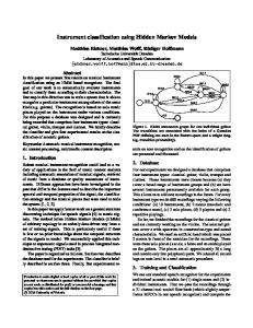
A. Warship All warships are designed and built to perform a common duty constitute a Type. In each type of warship, there are Classes or groups of ships built by the same design. If there is need for differentiation of classes this should left for reference into special charts, reference books or to those qualify by specialist study and who are right up to date with their knowledge [2]. The differences between the shapes of various ships mainly lie in their superstructures, while the differences of the shapes of ship bodies are little. Fig. 1 shows features coded of distant view of warship. To identify warship [11] codes the features of distant view as below: G : Gun Gs : Gun (small) C : Crane D : Director DR : Director (Raised) B : Bubble M : Mast F : Funnel L : Launcher

INTRODUCTION

The information technology for network-centric warfare (NCW) has a great level of importance for military decision operations. They need information management procedures to ensure that the right information is available for the right decider to make the right decision [1]. To classify an object as warship from a distant view is one of importance information. For ship recognition, many papers work on Inverse Synthetic Aperture Radar (ISAR) [2], [3], [4] and [5] and Forward Looking Infra-Red (FLIR) [6], [7] and [8] images. Some paper based on sonar images [9] and magnetic signature [10] for input data. To get ISAR, FLIR and sonar data images, we need big equipment that cannot fit for small vehicles or small aircrafts that need to move by high speed and work in operation field. Fortunately, with new technology we have the possibility to be capable for inserting small camera into small vehicles, aircrafts and robots to take picture and send the images back to be processed. This paper presents the algorithm to use distance view images from camera as input data to classify classes of warship and we present the difference of tangent-angles on superstructure boundary as descriptive feature. To classify warships that the superstructure of each class seems similar, we apply the dynamic time warping (DTW) for similar measures and this would speed up the computation by reducing size of the data set by the use of the piecewise aggregate approximation (PAA). The last process for robust classification, we used the k-nearest neighbor (k-NN) as classifier. This algorithm proved the quality of classification rate that invariant under translation scaling and rotation images.

The most important feature of recognition is the visual impact of hulls, masts, radar aerials, funnels and major weapons systems. There are nine sections which cover the major types of warships [11], namely: - Submarines - Aircraft Carriers - Cruisers - Destroyers - Frigates - Corvettes - Patrol Forces - Amphibious Forces - Mine Warfare Forces

Fig. 1. Example of features coded in the distant view of warship [11].

c 2012 IEICE. Permission request for reproduction: Service Department, Copyright ⃝ IEICE Headquarters Office, E-mail: [email protected]. IEICE Provisions on Copyright: http://www.ieice.org/eng/about/copyright.html.

150

RS3-4

2012 International Workshop on Smart Info-Media Systems in Asia (SISA 2012), Sep. 6–Sep. 8, 2012

(a) H.T.M.S. DAMYAT

and partial. The result has excellent recognition rates but data images need enough of details for the SIFT and computationally are very expensive. Alvaro Enriquez de Luna, Carlos Miravet, Deitze Otaduy and Dorronsoro [16] work with side view of silhouette of images by Curvature Scale Space (CSS) representation and compare by the Recursive Matching Matrix (RMM). The accuracy is close to 80% with viewpoint angle near 90 degrees variations within ± 10 degrees. The rotation which is larger than 10 degrees would be a misidentification. Our work used optical images as input data and our descriptive feature method was invariant for scaling translation and rotation.

(b) H.T.M.S. PHUTTHAYOTFA

Fig. 2. Warship type “Frigates” class “Knox”.

Each type of warship is classified to many classes and the superstructure of warship in each class is similar as show in Fig. 2. Many related works for warship classification have found. The early work for ship and warship classification, reference [12] use coordinates of contour turn points from silhouette‟s boundary. This method is variant under translation, scaling, rotation and noisy. Based on ISAR images, [2] use the Principal Components Analysis (PCA) shows the result as fair but it needs to be test with a large database. Reference [4] and [5] work with ISAR images but based on models, not on real data. Reference [6], Atle O Knapslog works on classify of Satellite synthetic Aperture Radar (SAR) images of ships in harbor and based on 3D models by measuring the distance between curves of the target and silhouette of 3D models. The result is good estimate if the ship is projected onto a sea background and the aspect angle is favorable. Real data from radar ship images are used for target recognition by M.R.Inggs and A.R. Robinson [13]. They use Fourier-Modified Discrete Mellin Transform (F-MDMT) to transform and compare with two classifiers, the first is backpropagation neural networks that require a long training times, the second is Learning Vector Quantization (LVQ) that is considered more favorable and classification accuracy is up to 93% for classify types of ship. Based on FLIR images, Qian zhongliang and Wang wenjun [7] use moment invariants as descriptive feature of superstructure of ship and 1-NN classifier, the results of the superstructure moment invariants as s descriptor has better discriminability and accuracy. Jorge Alves, Jessica Herman and Neil C. Rowe [8] report two experimental systems for ship classification, in an edge histogram approach obtain 80% accuracy and neural network approach. They use moment invariants as input to training in neural network. The accuracy is 85.4% in ship‟s types. However, the FLIR images need to eliminate common artifacts as ship shadows, reflections on the sea surface and heat from stacks. Ship classification based on covariance of discrete wavelet of ships image using probability neural network is present by Leila Fallah Araghi, Hamid Khaloozade and Mohammad Reza Arvan [9]. The classifier achieve 87.5% correct classification rate. Reference [14] M. Uma Selvi and S. Suresh Kumar presents ship recognition using color remote sensing imagery and obtaining a good classification rate. Optical image has used as input data for Scale Invariant Feature Transform (SIFT) [15] and measure the distance between vectors. That method is invariant to scaling, rotation

B. Dynamic Time Warping (DTW) The dynamic time warping algorithm is a well-known algorithm in many areas. While the first introduced by application to the speech recognition. It is currently used in many areas include data mining and time series [17]. DTW may be considers simply as a tool to measure the dissimilar between two time series, after aligning them. Suppose we have two time series Q and C, of length p and m, respectively, where: Q = q1,q2,…,qi,…,qp

(1)

C = c1,c2,…,cj,…,cm

(2)

In order to compare two different sequences Q and C one needs to use the local distance measure. The algorithm starts by building the distance matrix (p-by-m) representing all pairwise distances between C and Q. This distance matrix called the local cost matrix. Once the local cost matrix is built, the algorithm finds the alignment path that runs through the low-cost areas “valleys” on the cost matrix. Fig. 3 (Left) shows two time series sequences which are similar but out of phase and to align the sequences, we construct a warping matrix and search for the optimal warping path (solid squares). A band with width “r” is used to constrain the warping (Right). (a)

(c)

(b)

Time

W

Fig. 3. (a) Two similar time series Q and C. (b) A warping matrix and search for the optimal warping path (solid squares). (c) The resulting alignment.

151

RS3-4

2012 International Workshop on Smart Info-Media Systems in Asia (SISA 2012), Sep. 6–Sep. 8, 2012 design choices to make: the value of “k”, and the distance function to use. In order to avoid ties the most common choice for k is a small odd integer, for example k = 3. Ties can also arise when two distance values are the same. Usually, Euclidean distance is used as distance function, the Euclidean distance between xq and xi can be calculated as follows:

A warping path “W” is a contiguous set of matrix elements that defines a mapping between Q and C. The kth elements of W are defined as wk = (i, j)k as below: W = w1, w2, ...,wk,...,wK max(m, p) ≤ K ≤ m+p-1

(3)

The warping path must satisfy several constraints. 1) Boundary conditions: w1 = (1, 1) and wk = (p, m), this requires the warping path to start and finish in diagonally opposite corners. 2) Continuity: Given wk = (a, b) then wk-1 = (a', b') where a – a' ≤ 1 and b - b' ≤ 1. This restricts the allowable steps in the warping path to adjacent cells. 3) Monotonicity: Given wk = (a, b) then wk-1 = (a', b') where a – a' ≥ 0 and b - b' ≥ 0. This forces the points in W to be monotonically spaced in time. We interest in the path that minimizes the warping cost:

(6) Some papers work on k-NN with DTW for time-series classification [18], [19] and [22]. For our experimental, we used DTW for distance function instead of Euclidean. D. Piecewise Aggregate Approximation (PAA) To speed up the computation, [23] reduce the data from n dimensions to N dimensions by dividing the time series into N equal-sized „frames‟. The mean value of the data falling within a frame is calculated, and a vector of these values becomes the data reduced representation. The transformation produces a piecewise constant approximation of the original sequence, hence the name, Piecewise Aggregate Approximation (PAA). Keogh et al [23] suggest approximating a time series by dividing it into equal-length segments and recording the mean value of the data points that fall within the segment. This simple technique is surprisingly competitive with the more sophisticated transform [24]. Reference [23] speeds up DTW by modification to PAA with no loss of accuracy. Reference [25] also propose PAA can reduce the computational and turn increases the number of DTW calculations, the proposed PAA lower-bound estimate is able to speed up the overall DTW-k-NN search by 28%.

(4) This path can be found by using dynamic programming to evaluate the following recurrence which defines the cumulative distance γ(i, j) as the distance d(i, j) found in the current cell and the minimum of the cumulative distances of the adjacent elements:

γ(i, j) = d(qi, cj) + min {γ(i-1, j-1),γ(i-1, j),γ(i, j-1)} (5) The time cost of building this matrix is O(pm). In order to improve performance and customize the sensitivity of the “naive” Dynamic Time Warping algorithm various modification are proposed. The major modifications such as the step size conditions, step weighting and the global path constraints. In our experimental, to prove our descriptive feature, we follow on naive DTW as shown in [17] and one-nearestneighbor using dynamic time warping (1NN-DTW) that seems to be the best approach for time series classification [18] and [19].

E. Contour Tracing The goal of contour tracing is to find an external contour at a given pixel, named S. At this pixel, we first execute Tracer. If Tracer identifies S as an isolated pixel, we reach the end of Contour Tracing. Otherwise, Tracer will output the next contour point of S. Let name this point T. We then continue to execute tracer to find the next contour point of T, then its next point, etc. until the following two conditions hold: (i) Tracer outputs S again, and (ii) the next contour point of S is T again and the procedure would stop only when both of the above conditions hold. Reference [29] obtains geometrical shapes information and edge points of objects.

C. k-Nearest Neighbor (k-NN) Supervised learning is the most fundamental task in machine learning. In supervised learning, we have training examples and test examples. A training example is an ordered pair (x, y) where x is an instance and y is a label. A test example is an instance x with unknown label. The goal is to predict labels for test examples [20]. One example for an instance-based learning algorithm is the k-Nearest Neighbor (k-NN) algorithm. It uses the k-nearest neighbors to make the decision of class attribution directly from the training instances themselves. The decision for attaching the sample in question to one of the several classes is based on the majority vote of its k-nearest neighbors. An odd number should be chosen for k to allow for a definite majority vote [21]. The k-NN method is perhaps the simplest of all algorithms for predicting the class of a test example. There are two major

III.

METHOD

A. Data and Preprocessing For our experiment, we used silhouettes of warship from Jane‟s Fighting Ship 2010 – 2011 [26] and Jane‟s Warship Recognition Guide [27] as input data images. The preprocessing only removed the background from images. Fig. 4 shows general concept of algorithm for warship classification.

152

RS3-4

2012 International Workshop on Smart Info-Media Systems in Asia (SISA 2012), Sep. 6–Sep. 8, 2012 was the number of boundary pixels for the region. Matrix held the row and column co-ordinates of the boundary pixels. The co-ordinate of pixels of outer boundary is:

Preprocessing

Q = (X1,Y1), (X2,Y2),….. (Xn,Yn)

(7)

ROI selection

Instead of using co-ordinate, we used tangent angle as shape representation and description. We applied algorithm of [30] and [31] by calculated tangent in degree angle. With this algorithm, translation position of image can be extract with the same feature. The tangent angle was invariant with change of scale, also with calculation tangent in degree we can fixed the tangent of π/2 and 3π/2 that not defined in radian. The tangent between two co-ordinates is:

Extraction

Classification

Tn = (Yn+1 – Yn) / (Xn+1 – Xn)

(8)

To translate from radians to degrees, we recall the con version rules: radian * (180/π). The set of tangent is:

Fig. 4. General concept of algorithm for warship classification.

B. Translation Scaling and Rotation Feature Extraction Our method started with extracted the superstructure of image by transform image to binary image and calculated difference of tangent along boundary of binary image. To fixed the Region-of-interest (ROI) and avoided noisy, the ratio and PAA method gave average angles to DTW and kNN work with difference of tangent data for classification, the detail as below. Step 1: Transformed image to binary image. In binary image, “0” instead of black or object area and “1” instead of white or background area. Step 2: Region-of-interest (ROI), to find the boundary by Contour Tracing [28]. The goal of contour tracing was to find an external contour at a given pixel, named S. At this pixel, we first executed tracer. If tracer identified S. as an isolated pixel, we reach the end of Contour Tracing. Otherwise, tracer will output the next contour point of S. Let name this point T. We then continue to executed tracer to find the next contour point of T, then its next point, etc. until the following two conditions hold: (i) tracer outputs S again, and (ii) the next contour point of S was T again and the procedure would stop only when both of the above conditions hold. Reference [29] obtains geometrical shapes information and edge points of objects. We followed [28] and [29] to get outer boundary of images.

T = (T1, T2, T3,..,Tn)

(9)

Rotation Step 4: To work with rotation, we calculated the set of difference of tangent and used as the description defined as follows: DTn = ( Tn+1, - Tn) DTS = (DT1, DT2, DT3 ,.., DTn)

(10) (11)

DT was difference of tangent in each tangent point and DTS was set of DT. Step 5: We applied PAA to reduce the data dimension that can speed up the distance function, as shown in Fig. 6. The formula for average of angle of tangent in length “n” was show below. Davg = ((DT1+ DT2+ DT3 +….. + DTn) /n)

(12)

Dpaa = (Davg1, Davg2, Davg3 ,….. , Davgn)

(13)

Davg was an average of tangent of length “n” and Dpaa was set of Davg that we extract from ship silhouette. We used Dpaa as data for distance function (DTW) and classified by k-NN for Similar Measured and Classification Section.

Fig. 5. Ship silhouette (left) and its boundary (right).

Translation and Scaling Step 3: Outer boundary of binary image as show in Fig. 5 from Step 2 that contour tracing algorithm in eight-connected binary images, this function returns a Q-by-2 matrix, where Q Fig.6. The Difference of Tangent and its PAA

153

RS3-4

2012 International Workshop on Smart Info-Media Systems in Asia (SISA 2012), Sep. 6–Sep. 8, 2012

C.

Similar Measure and Classification Since we had set of averages of difference of angle of tangent (Dpaa) that invariant for translation scaling and rotation, now we can measured the similar between the ship that we know and the other one that we did not know its class. DTW was used for distance measure and gave the similar order for k-NN to classify the unknown ship. D.

Basic concept Fig. 7 shows that the data from tangent angle function from three geometry images had difference angle because of translation rotation and scaling images ((a), (b), (c)) as plot the tangent angle shown in (d). When we used the difference of angle, the output data were similar as shown in (e).

Fig. 8. Example of warship images.

IV. (a) Original

(b) Rotation

(c) Scaling

EXPERIMENTAL EVALUATION

This section describes the results of the experiments. A. Dataset For experiment, we test our method with images of 8 types, 68 classes of warship in original, reduced by size and rotated images. Fig. 8 shows the example is for warship images. B. Experiment result The result of our experiment can prove that our method had good classification rate under translation, scaling and fairly for rotation in each class of ships. Table I. shows comparing classification rate result between Euclidean (ED) and DTW with 1-NN. The average of DTW classification rate is 81.86% and ED rate is 50.49%. We found that DTW and ED gave near classification rate under translation. However, DTW gave more robust classification rate than ED under scaling and rotation.

(d) Tangent angle with PAA

TABLE I RESULT OF CLASSIFICATION RATE (%) Types of Warships Amphibious Aircraft Carriers Corvettes Cruisers Destroyers Frigates Mine Warfare Patrol Forces Average

(e) Difference of tangent angle with PAA Fig. 7 Difference of tangent angle with PAA is invariant for translation rotation and scaling.

154

Translation

Scaling

Rotation

DTW

ED

DTW

ED

DTW

ED

100 100 100 100 100 100 100 100 100

100 100 100 100 100 100 100 100 100

100 88.89 75.00 90.00 83.33 66.67 50.00 80.00 79.41

0.00 0.00 33.33 10.00 66.67 11.11 16.67 40.00 25.00

60.00 66.67 66.67 70.00 66.67 44.44 100.00 60.00 66.18

20.00 22.22 25.00 10.00 58.33 33.33 0.00 20.00 26.47

RS3-4

2012 International Workshop on Smart Info-Media Systems in Asia (SISA 2012), Sep. 6–Sep. 8, 2012 [17] P. Senin, Dynamic Time Warping Algorithm Review, Honolulu, Hawaii: University of Hawaii at Manoa, 2008. [18] X. Xi, E. Keogh, C. Shelton, L. Wei, “Fast Time Series Classification Using Numerosity Reduction”, International Conference of Machine Learning, Pittsburgh, PA, 2006. [19] K. T. Islam, K. Hamrul, Y. Lee, S. Lee, “Enhanced 1-NN Time Series Classification Using Badness of Records”, in Proc. ICUIMC, Suwon, South Korea, 2008. [20] C. Elkan, Nearest Neighbor Classification, UCSD, 2011. [21] M. Weis, T. Rumpf, R. Gerhards, L. Plumer, “Comparison of different classification algorithms for weed detection form images based on shape parameters”, Dep. Of Weed Science, University of Hohenheim, Germany, 2009. [22] H. Hsu, A. C. Yang, M. Lu, “KNN-DTW based Missing Value Imputation for Microarray Time Series Data”, Journal of Computers, Vol.6 No.3, 2011, pp.418-425. [23] E. J. Keogh, M. J. Pazzani, Scaling up Dynamic Time Warping for Data mining Applications, Irvine, CA: University of California, 2000. [24] C. A. Ratanamahatana, J. Lin, D. Gunopulos E. Keogh, Mining Time series Data, Riverside, CA: University of California. [25] Y. Zhang, J. Glass, “A piecewise Aggregare Approximation Lower-Bound Estimate for Posteriorgram-based Dynamic Time Warping”, ISCA, Florence, Italy, 2011, pp.1909-1912. [26] S. Saunders, Jane‟s Fighting Ships 2010-2011. [27] Anthony J. Watts. Jane‟s Warship Recognition Guide. New York, NY: Collins, 2006. [28] F. Chang, C. Chen, “A Component-Labeling Algorithm Using Contour Tracing Techique”, IEEE Transactions on Document Analysis and Recognition, 2003. [29] M. F. Talu, I. Turkoglu, “A Novel Object Recognition Method Based on Improved Edge Tracing for Binary Images”, IEEE,2009. [30] F. Feschet, L. Tougne, “Optimal Time Computation of the Tangent of a Discrete Curve:Application to the Curvature”, DGCI,LNCS 1568,Bron cedex, France, 1999, pp.31-40. [31] J. Matas, Z. Shao, J. Kittler, “Estimation of Curvature and Tangent Direction by Median Filtered Differencing”, Int. Conf. on Image Analysis and Processing, San Remo, 1995, pp.13-15.

V. CONCLUSIONS Our work present difference of tangent-angle, algorithm for feature extraction that can measured feature similar of translation scaling and rotation object. We applied this algorithm to warships that each class is very similar. Our experiment proved that this method can gave us the good classification result when applied to DTW and k-NN. For future work, to apply an elaboration with online classification we will need more speed up the DTW and we can apply this algorithm to partial of object or other object recognition. ACKNOWLEDGMENT This Work is Supported by the 60th Year Supreme Reign of his Majesty King Bhumibol Adulyadej Scholarship, granted by the Faculty of Graduate Studies Academic Year 2011, Mahidol University. REFERENCES [1] S. Renner, “Building Information Systems for Network-Centric Warfare”, The MITRE Corporation, MA, 2003. [2] V. Gouaillier, L. Gagnon, “Ship Silhouette Recognition Using Principal Components Analysis”, SPIE Proc. #3164, CA, 1997. [3] D. pastina, C. Spina, “Multi-feature based automatic recognition of ship targets in ISAR images” IEEE, University of Rome, 2008. [4] F. Rice, T. Cooke, D. Gibbins, “Model based ISAR ship classification”, Digital Signal Processing 16, 2006, pp.628-637. [5] A. O. Knapskog, “Classification of Ships in TerraSAR-X Images Based on 3D Models and Silhouette Matching”, EUSAR, Norway, 2010. [6] Q. Zhongliang, W. Wenjon, “Automatic Ship Classification by Superstructure Moment Invariants and Two-stage Classifier”, ICCS/ISITA, Singapore, 1992, pp. 544-547. [7] J. Alves, J. Herman, N. C. Rowe, “Robust Recognition of Ship Types from an Infrared Silhouette”, Naval Postgraduate School, CA, 2004. [8] L. F. Araghi, H. Kholooade, M. R. Arvan, “Ship Identification Using Probabilistic Neural Network(PNN)”, IMECS, 2009, pp.326-329, [9] V. J. Lobo, N. Bandeira, F. Moura-Pires, “Ship recognition using Distributed Self Organizing Maps”, EANN 98, PORTUGAL, 1998. [10] J. A. Arantes do Amaral et al., “Ship‟s Classification by its Magnetic Signature”, IEE International, 1998. [11] Talbot-Booth, David Greenman, Warship Identification. United States Naval Institute, Maryland: Annapolis, 1971. [12] M. J. Bizer, “A Picture-descriptor Extraction Program Using Ship Silhouettes”, DTIC, Monterey, CA, 1989. [13] M. R. Inggs, A. R. Robinson, “Neural Approaches to Ship Target Recognition”, IEEE International Radar Conference, 1995, pp.386-391. [14] M. U. Selvi, S. S. Kumar, “A Novel Approach for Ship Recognition using Shape and Texture”, IJAIT Vol.1 No.5, 2011, pp.23-28. [15] P. A. Feineigle, D. D. Morris, F. D. Snyder, “Ship Recognition Using Optical Imagery for Harbor Surveillance”, AUVSI, Washington DC, 2007. [16] A. E. Luna, et al., “A decision support system for ship identification based on the curvature scale space representation”, Madrid, Spain, 2005.

155